Geospatial Triangle Example

In this example we’ll illustrate how to generate a mesh from a “real-world” geospatial vector dataset.

import geopandas as gpd
import matplotlib.pyplot as plt
import pandas as pd
import shapely.geometry as sg

import pandamesh as pm

Overlap

We will get the data of a GeoJSON file describing the provinces of the Netherlands, and select only the name and geometry columns. We’ll set the coordinate reference system to the Dutch national standard (EPSG:28992). Finally we set the name column to be used as index, so we can select provinces on name.

provinces = pm.data.provinces_nl().loc[:, ["name", "geometry"]]
provinces = provinces.to_crs("epsg:28992")
provinces.index = provinces["name"]
gdf = provinces.copy()

The mesh generation software cannot deal with overlap of polygons. To get rid of overlap, we can use the spatial functionality that geopandas provides. Let’s check the polygons for overlap first.

overlap = gdf.overlay(gdf, how="intersection", keep_geom_type=True)
overlap = overlap.loc[overlap["name_1"] != overlap["name_2"]]

fig, ax = plt.subplots()
gdf.plot(ax=ax)
overlap.plot(edgecolor="red", ax=ax)

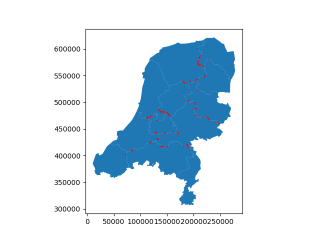
<Axes: >

Clean-up

There are many small overlaps visible at the province borders.

We can generate a consistent polygon using a unary union.

union = sg.Polygon(gdf.unary_union)
union_gdf = gpd.GeoDataFrame(geometry=[union])
union_gdf["cellsize"] = 10_000.0

Unfortunately, the province boundaries of this dataset no do align neatly and there are a number of small holes present. Some of these holes are not formed by inconsistencies, but by a small number of Belgian exclaves, Baarle-Hertog.

Simplify

We’ll ignore the subtleties of international law for now and use geopandas to remove all blemishes by:

• squeezing out the holes with .buffer

• dissolving the buffered polygons into a single polygon with .dissolve

• simplifying the dissolved polygon to avoid over-refinement with .simplify

This creates a clean, and simpler, geometry.

simplified = gdf.copy()
simplified.geometry = simplified.geometry.buffer(500.0)
simplified["dissolve_column"] = 0
simplified = simplified.dissolve(by="dissolve_column")
simplified.geometry = simplified.geometry.simplify(5_000.0)
simplified["cellsize"] = 10_000.0

simplified.plot()

<Axes: >

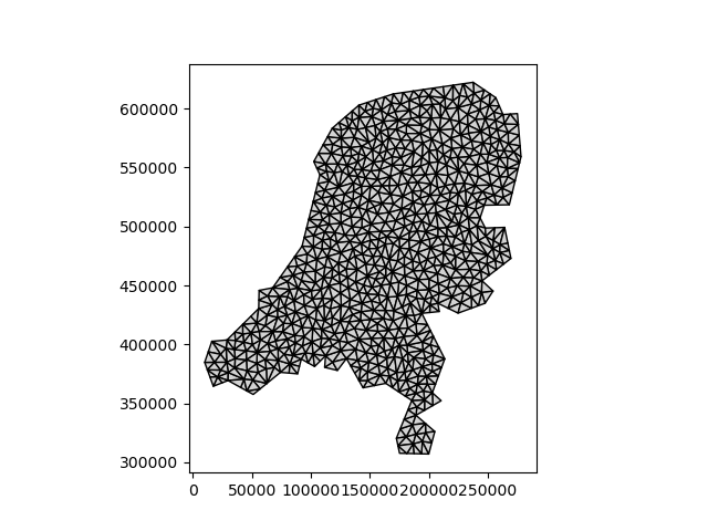
Using this clean geometry, we can generate an unstructured grid with a fairly constant cell size.

mesher = pm.TriangleMesher(simplified)
vertices, triangles = mesher.generate()
pm.plot(vertices, triangles)

Local refinement

To set a zone of refinement, we can define an additional polygon. We need to ensure that no overlap occurs in the follwing steps:

• select the geometry of a single province;

• simplify its geometry to an appropriate level of detail;

• specify a smaller cell size;

• remove this province from the enveloping polygon;

• collect the two polygons in a single geodataframe.

utrecht = gdf.loc[["Utrecht"]]
utrecht.geometry = utrecht.geometry.simplify(2_500.0)
utrecht["cellsize"] = 5000.0

envelope = simplified.overlay(utrecht, how="difference")
refined = pd.concat([envelope, utrecht])
refined.index = [0, 1]
refined.plot(column="name")

<Axes: >

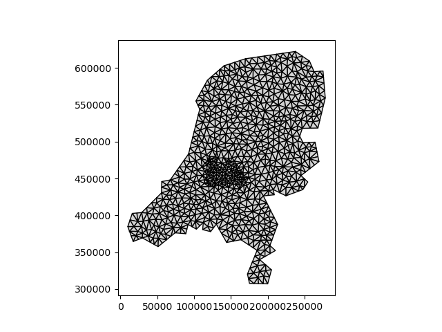
This results in a mesh with a smaller cell size in the province of Utrecht.

mesher = pm.TriangleMesher(refined)
vertices, triangles = mesher.generate()
pm.plot(vertices, triangles)

Conclusion

This example provides a taste of how to convert a geospatial vector dataset into an unstructured grid with a locally refined part. Real-world data generally come with their own idiosyncrasies and inconsistencies. Depending on the nature of the necessary fixes, they can be solved with geopandas functionality, but sometimes manual editing is required. Fortunately, geopandas provides easy input and output for many file formats, which can be opened by e.g. QGIS.