Gmsh Fields Example

Gmsh supports so called “fields” to guide the cell sizes of the generated meshes. These fields are separate from the geometrical constraints: for example, a field point does not end up in the generated mesh, but influences the cell size in its surrounding.

These field geometries can be added via:

• pandamesh.GmshMesher.add_threshold_distance_field()

• pandamesh.GmshMesher.add_matheval_distance_field()

• pandamesh.GmshMesher.add_structured_field()

• pandamesh.GmshMesher.add_structured_field_from_dataarray(),

The examples below demonstrate how to set up these distance fields for meshing.

import geopandas as gpd
import matplotlib.pyplot as plt
import numpy as np
import shapely.geometry as sg

import pandamesh as pm

Point fields

We’ll start again with simple rectangular example.

polygon = sg.Polygon(
    [
        [0.0, 0.0],
        [10.0, 0.0],
        [10.0, 10.0],
        [0.0, 10.0],
    ]
)
point = sg.Point([4.0, 4.0])
gdf = gpd.GeoDataFrame(geometry=[polygon])
gdf["cellsize"] = 5.0

mesher = pm.GmshMesher(gdf, shift_origin=False)
mesher.mesh_size_extend_from_boundary = False
mesher.mesh_size_from_curvature = False
mesher.mesh_size_from_points = False

pm.plot(*mesher.generate())

Threshold distance fields

Gmsh supports changing cell sizes gradually, for example as a function of distance to a feature. We can add a point, and connect a distance threshold field to it:

point = sg.Point([4.0, 4.0])
field = gpd.GeoDataFrame(geometry=[point])
field["dist_min"] = 2.0
field["dist_max"] = 4.0
field["size_min"] = 0.5
field["size_max"] = 2.5
field["spacing"] = np.nan
mesher.add_threshold_distance_field(field)

vertices, faces = mesher.generate()
pm.plot(vertices, faces)

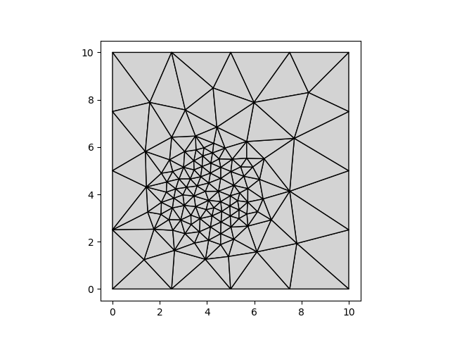
Within the dist_min of the point, all cell sizes have size of at most size_min. This changes linearly until dist_max is reached, at which point the cell sizes become size_max.

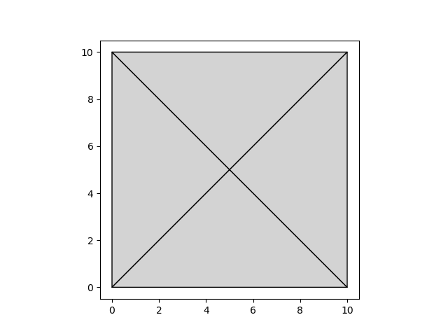
Fields can be removed via .clear_fields():

mesher.clear_fields()
vertices, faces = mesher.generate()
pm.plot(vertices, faces)

Gmsh only measures distances to point. The spacing is used to interpolate points along lines:

mesher.clear_fields()

line = sg.LineString(
    [
        [3.0, -3.0],
        [3.0, 13.0],
    ]
)
field = gpd.GeoDataFrame(geometry=[line])
field["dist_min"] = 2.0
field["dist_max"] = 4.0
field["size_min"] = 0.5
field["size_max"] = 2.5
field["spacing"] = 2.0
mesher.add_threshold_distance_field(field)

vertices, faces = mesher.generate()
pm.plot(vertices, faces)

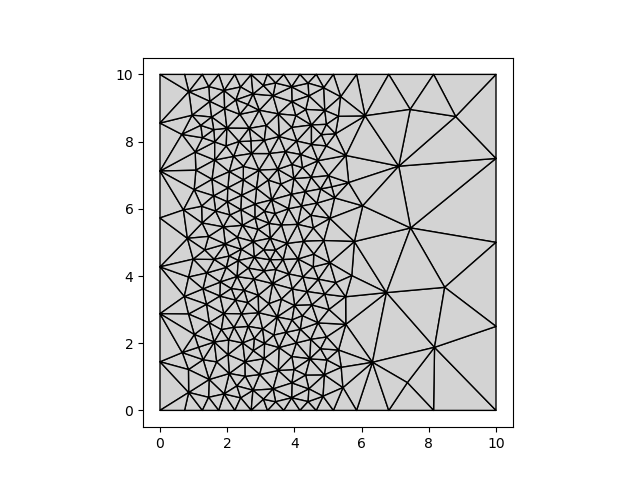
Note that unlike the mesher input geometries, these geometries may fall outside the meshing domain: they only “radiate” a cell size.

Polygons can also be used as field geometries. Distances are measured from internal and external boundaries:

mesher.clear_fields()

square = sg.Polygon(
    [
        [3.0, 3.0],
        [7.0, 3.0],
        [7.0, 7.0],
        [3.0, 7.0],
    ]
)
field = gpd.GeoDataFrame(geometry=[square])
field["dist_min"] = 0.5
field["dist_max"] = 1.5
field["size_min"] = 0.3
field["size_max"] = 2.5
field["spacing"] = 1.0
mesher.add_threshold_distance_field(field)

vertices, faces = mesher.generate()
pm.plot(vertices, faces)

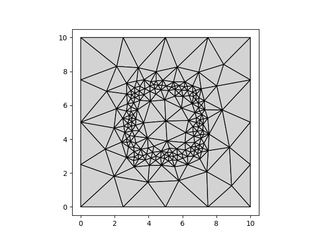
MathEval distance fields

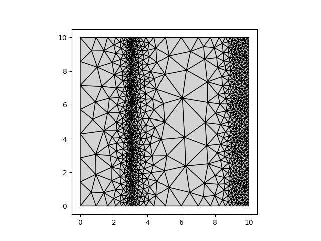
Gmsh also supports arbitrary mathematical functions. With Pandamesh, these can be easily combined to specify cell size a function to some boundary. For example, we can specify cell size as quadratically growing with the distance from the left boundary:

mesher.clear_fields()

line = sg.LineString(
    [
        [0.0, 0.0],
        [0.0, 10.0],
    ]
)
field = gpd.GeoDataFrame(geometry=[line])
field["function"] = "distance^2 + 0.3"
field["spacing"] = 1.0
mesher.add_matheval_distance_field(field)

vertices, faces = mesher.generate()
pm.plot(vertices, faces)

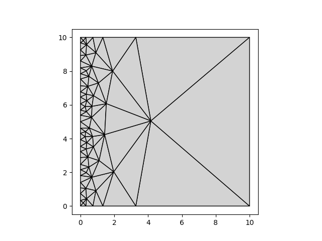
Note that we should take care to specify a function which is always larger than zero in the meshing domain.

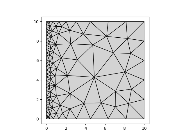
Unlike input geometries, fields can be added in a piece by piece manner. The distance is always relative to the feature of the geometry in the GeoDataFrame row.

second_field = gpd.GeoDataFrame(geometry=[sg.Point([5.0, 5.0])])
second_field["function"] = "max(1/(distance^2), 2.0)"
second_field["spacing"] = np.nan
mesher.add_matheval_distance_field(second_field)

vertices, faces = mesher.generate()
pm.plot(vertices, faces)

Structured fields

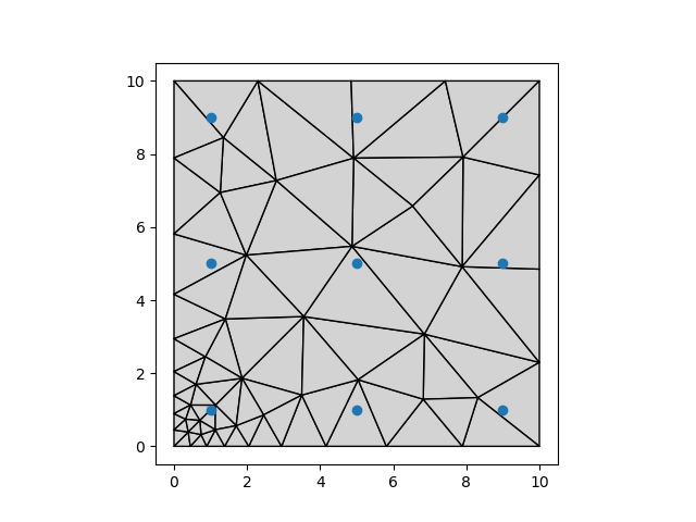
In some cases, the generated cell size should depend on some physical properties of the domain. In geospatial applications, such properties are often represented as raster data. These data can be used to guide mesh generation as a structured grid. The cell size is prescribed at the grid points, and interpolated between.

In the example below, we generate 3 by 3 grid of cell sizes, with small cell sizes in the lower left corner, and large cell sizes in the upper right:

mesher.clear_fields()

y, x = np.meshgrid([1.0, 5.0, 9.0], [1.0, 5.0, 9.0], indexing="ij")
distance_from_origin = np.sqrt((x * x + y * y))
cellsize = np.log(distance_from_origin / distance_from_origin.min()) + 0.5
mesher.add_structured_field(
    cellsize=cellsize,
    xmin=x.min(),
    ymin=y.min(),
    dx=1.0,
    dy=1.0,
)
vertices, faces = mesher.generate()

fig, ax = plt.subplots()
pm.plot(vertices, faces, ax=ax)
ax.scatter(x, y)

<matplotlib.collections.PathCollection object at 0x7f48224a61e0>

DataArray structured fields

These structured fields can also be provided as xarray DataArrays:

mesher.clear_fields()

import xarray as xr

x = np.arange(1.0, 10.0)
y = np.arange(1.0, 10.0)
da = xr.DataArray(np.ones((y.size, x.size)), coords={"y": y, "x": x}, dims=("y", "x"))

mesher.add_structured_field_from_dataarray(da)
vertices, faces = mesher.generate()
pm.plot(vertices, faces)

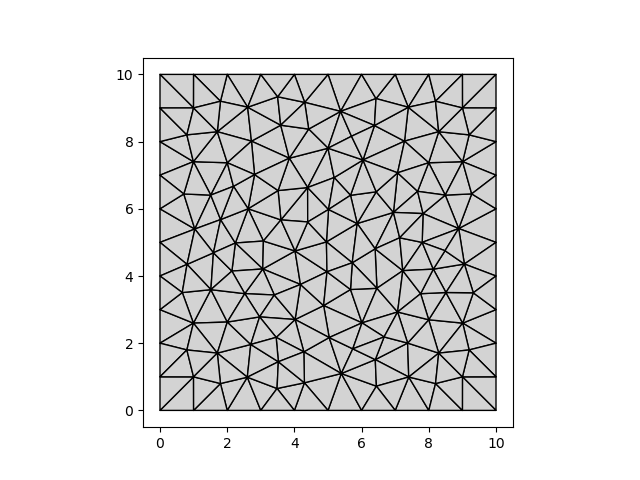
This is arguably the most flexible way of configuring cell sizes, since we can easily modify the DataArray values. Note that like the MathEval specification, we need to take care to ensure values remain > 0.

mesher.clear_fields()

cos_da = da * np.cos(da["x"]) + 1.1
mesher.add_structured_field_from_dataarray(cos_da)
vertices, faces = mesher.generate()
pm.plot(vertices, faces)