Frequently asked questions
How do I easily modify input parameters?
See this section on how to adjust maps, and this section on how to directly pass uniform values. Note that both options work for any parameter.
How do I start wflow with initial conditions from a previous run?
See here
How do I add external inflows and/or abstractions?
river_water__external_inflow_volume_flow_rate: positive for inflows, negative for abstraction. If parameter is time varying, add it to the correct section, see below. Note that these values can only be specified on river cells.
How do I add time-varying parameters?
Either through cyclic (add parameter to cyclic list in the toml), or to the forcing section.
How do I add different output?
See here for csv output, here for scalar netcdf data, and here for gridded netcdf output.
Which river routing option should I choose?
The choice of a specific river routing option can vary depending on the model and use case. However, the numerical properties of the routing schemes provide an indication of their advantages and disadvantages. The following river routing schemes are available:
- Kinematic wave
- Mannings flow on a staggered grid
- Local inertial routing on a staggered grid
These routing schemes support an optional 1D floodplain schematization (routing is done separately for the river channel and floodplain).
The kinematic wave method is driven by the river slope within each cell, assuming that the water surface slope is parallel to the bed slope. This results in sharper discharge peaks with minimal damping, as the waves travel through the system without deformation. This approach is especially suitable for steep (upstream) areas where flow propagation is dominated by topography. The kinematic wave approach does not include any form of backwater effects.
As the kinematic wave method, the use of Manning’s equation on a staggered grid is also driven by the river slope and thus most suitable for steep terrain where backwater effects are negligible.
On the other hand, the local inertial method incorporates the slope of the water surface into the momentum equation. This results in ‘damping effects’ on flow propagating through the cells and yields better results in scenarios where the water surface slope differs from the bed slope. This is particularly relevant in flat (downstream) regions where the river slope is limited or during the propagation of larger flood waves where the water surface slope is greater than the river slope itself. The local inertial method does incorporate backwater effects, although not as comprehensively as the full dynamic wave equation.
Generally, the kinematic wave method and the use of Manning’s equation on a staggered grid is computationally faster than the local inertial method for river (and land) routing. For the multi-threading execution of the kinematic wave, solved with a nonlinear scheme using Newton’s method, the order of execution (sub-basins) is important (from upstream to downstream sub-basin). For the momentum equation of river flow on a staggered grid an explicit numerical method is used and can be solved independently for each cell during multi-threading execution. As a consequence, speedups for river flow on a staggered grid are larger than for kinematic wave routing using multi-threading (compared to a single thread run) and the difference between river flow on a staggered grid and kinematic wave routing run times gets smaller as the number of threads increase.
Which land routing option should I choose?
Similar to river routing, the selection of the type of land routing depends on the model and use case. In practice, the kinematic wave approach is often sufficient for land routing. When the kinematic wave approach is used, water can flow from land cells into river cells, but not the other way around. The local inertial method for land routing is considered in cases where routing occurs over very flat areas or where complicated inundation patterns need to be included in both land and river routing.
The computational differences between the two options are larger than those between river routing options. This is due to the fact that there are typically more land cells than river cells in a model, and that for local inertial land routing two momentum equations (in the x and y direction) need to be solved. Consequently, more equations (with a higher computational cost compared to the kinematic wave method) must be solved compared to the combination of kinematic wave for land routing and local inertial for river routing.
What is the difference between 1D, 2D and no floodplains?
Effects of floodplain flow can be included in several ways. A one-dimensional sub-grid approximation (hence the name 1D floodplains) can be included when kinematic wave land routing is combined with river routing. The water surface elevations of the river channel and the floodplain are the same and it is assumed that water is exchanged instantaneously between the river channel and the floodplain. When the water depth in the river channel rises above the river bankfull depth, water is exchanged between the river channel and the floodplain resulting in an attenuation of the discharge peaks.
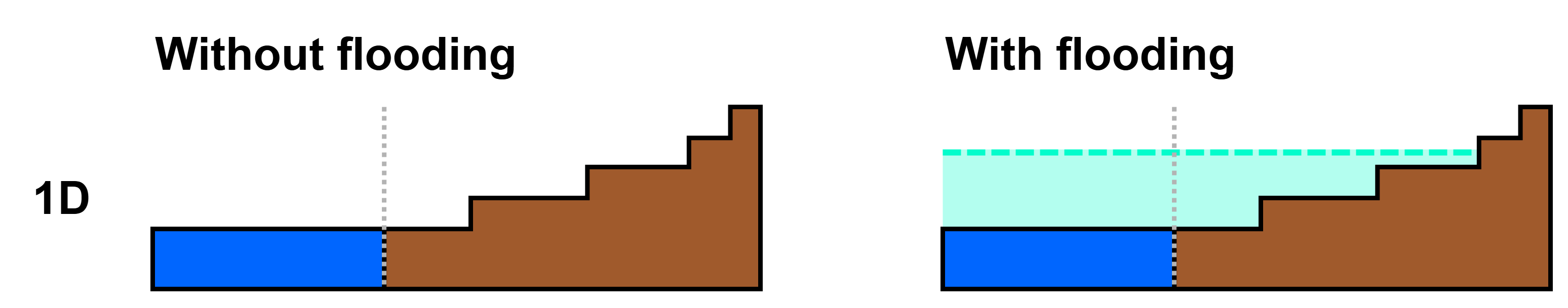
Routing is done separately for the river channel and floodplain, and using this feature does result in larger computational times.
Also for the local inertial approximation of both land and river routing, the water surface elevations of the river channel and the associated land cell (floodplain) are the same and is it assumed that water is exchanged instantaneously between the river channel and associated land cell (floodplain). Between land cells water can flow in two directions (x and y direction) hence the term 2D floodplain method. Additionally, saturation‐excess and infiltration‐excess overland flow are routed in two directions. Note that overland flow can not occur diagonally as opposed to the river routing, which may overestimate flow paths near river cells. Furthermore, as water from the river is exchanged with the full land cell the inundation area can be overestimated, especially for small river channels or land cells with relatively large sub-grid elevational differences. If these limitations are not acceptable, the 1D floodplain method can be used instead.
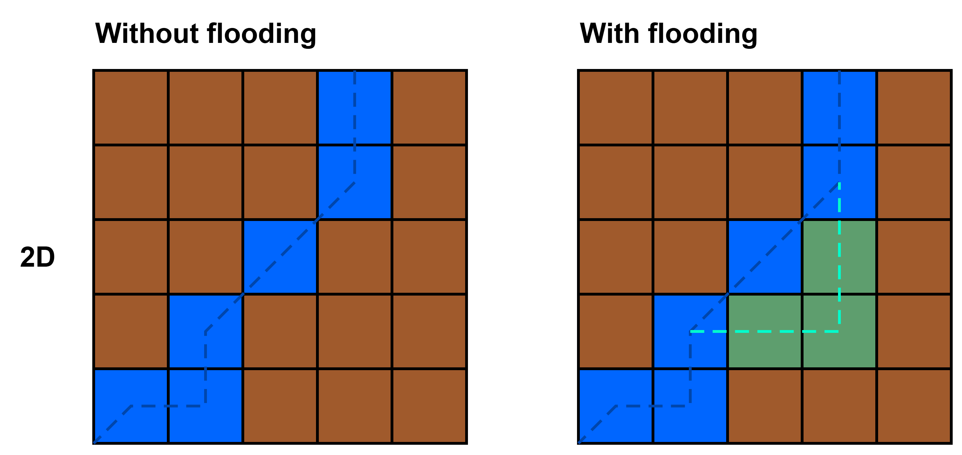
It is also possible to run the model without 1D floodplains. This can lead to unrealistically large water depths when the bankfull capacity is exceeded as there is no exchange of water between the river channel and floodplains.
How do I run only a part of my model?
You can easily run only a subsection of your model, by modifying the subbasin_location__count to a different layer in your staticmaps. By default, this layer represents your entire catchment, and all cells that have a value are interpreted as active cells. You can update this to another layer which contains a subset of the original data.
Alternatively, you can point subbasin_location__count to a layer with subcatchment information (e.g. based on gauges with discharge observations), and use the subbasin_active_location__count setting to provide a list of IDs within that layer that indicate the basins that you want to simulate. See below for an example:
[input]
subbasin_location__count = "subcatchment_gauges_obs"
subbasin_active_location__count = [1016, 1013, 1011, 206, 203, 503]When using this functionality, please take the following points into account:
- Ensure that all upstream regions are included (unless you make use of external inflows)
- When using water demand and allocation: ensure that there are no allocation areas with the same ID outside your active domain (a warning is shown in the logging)
- When writing output at specific cells (
index): note that the targeted cell (or e.g. reservoir) might no longer be at the same (active) index when using a different domain. If you need output at specific locations, please connect to a layer in the staticmaps, or provide coordinates. - When using local_inertial for routing: a ghost node will be added at the end of each river section (with a set distance and water level). This might cause some difference in the results, as it no longer contains the “real” downstream boundary condition. If this is important, either add a boundary condition at these locations (via
model_boundary_condition_river__lengthandmodel_boundary_condition_river_bank_water__depth), or ensure that the gauges for evaluation have sufficient downstream cells in your selected model domain. - Especially when running the
sbm_gwfmodel or using “local_inertial” forland_routing, please be aware that your active model domain covers the full relevant hydrologically active area, as this can be slightly different than e.g. typical subcatchment (elevation derived) maps.