QGIS plugin
1 How to
1.1 Start
Install QGIS version 3.28 or higher.
1.1.1 Install Ribasim plugin
Download ribasim_qgis.zip, see the download section.
Plugins menu > Manage and Install Plugins…
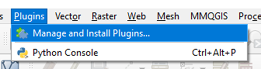
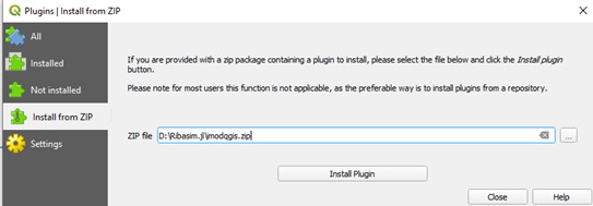
Select “Install from ZIP”:
- Browse to the
ribasim_qgis.zipfile containing the plugin that was downloaded earlier - Click “Install Plugin”
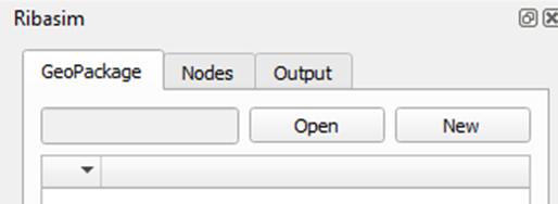
Start the Ribasim plugin.

1.1.2 Add iMOD plugin
In QGIS, navigate to “Plugins > Manage and Install Plugins > All”. In the search bar, type: “iMOD”. Select the iMOD plugin, and click “Install”.
At least version 0.4.0 of the iMOD plugin is required.
The Time Series widget from the iMOD plugin is used for visualizing Ribasim results, which is described in Section 1.5. Documentation on the Time Series widget can be found in the iMOD documentation.
1.1.3 Prepare your model
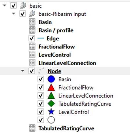
Open an existing model or create a new model. As an example of an existing model, you can use the “basic” model from generated_testmodels.zip, see the download section.
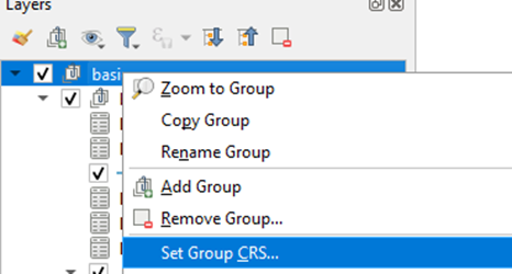
Check if your coordinate reference system (CRS) is set correctly.
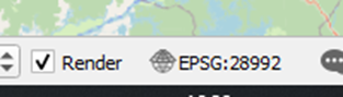
If you are working with an unknown CRS, right click the model database group in Layers, and click “Set Group CRS…”.
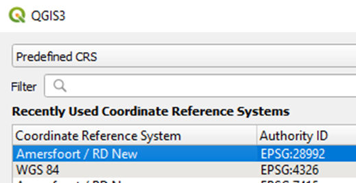
If you are modeling the Netherlands, select “Amersfoort / RD New” (EPSG:28992).
1.2 Edit nodes
1.2.1 Add nodes on the map
Select the Node layer.
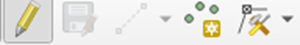
Turn on the edit mode to be able to add nodes on the map.
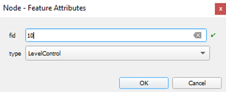
Add nodes to the map with a left click and select the node type.
Turn the edit mode off and save the edits to the Nodes layer.

1.2.2 Edit tables
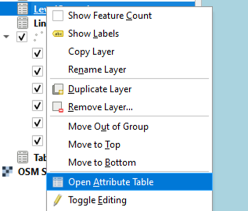
Right click a layer and select “Open Attribute Table”.
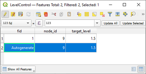
Click the yellow pencil icon on the top left to enable editing, and copy and paste a record. A record can be selected by clicking on the row number.
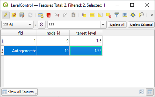
Adjust the content. If you prefer, it also works to copy data with the same columns from Excel. Turn off edit mode and save changes to the layer.
1.3 Connect nodes
1.3.1 Turn on snapping
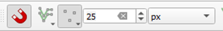
Make sure the Snapping Toolbar is visible, by going to the View > Toolbars menu. Turn on snapping mode by clicking the magnet and set the snapping distance to 25 pixels.
1.3.2 Create connecting edges
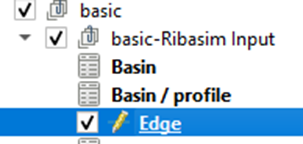
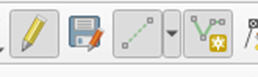
Select the Edge layer and turn on the edit mode.
Select “Add line feature”.
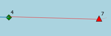
Create a connection by left clicking a source node and right clicking the destination node.
Now leave the edit mode and save the results to the layer.
1.4 Run a model
- Unzip the Ribasim command line interface,
ribasim_cli.zip - Open your terminal and go to the directory where your TOML is stored. Now run
path/to/ribasim_cli/ribasim ribasim.toml. Adjust the path to theribasim_clifolder to where you placed it. This runs the model. - In your model directory there is now a
results/folder withbasin.arrowandflow.arrowoutput files.
1.5 Inspect results
Before trying to inspect the results, verify that the run was successful and the output files are there.
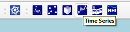
Click the “Time Series” button of the iMOD plugin.
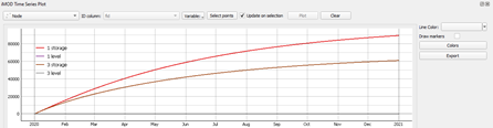
Select the layer that you wish to plot. From the “Node” layer you can plot level or storage on Basin nodes. From the “Edge” layer you can plot flow over flow edges. Note that before switching between these, you typically have to click “Clear” to clear the selection. If you run a simulation with the model open in QGIS, you have to close and re-open the “iMOD Time Series Plot” panel for the new results to be loaded.
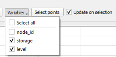
Select the variables that you want to plot.
Click “Select points” and select a node by dragging a rectangle around it on the map. Hold the Ctrl key to select multiple nodes.
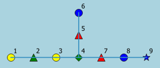
The associated time series are shown the the graph.
Only the “basin.arrow” and “flow.arrow” can be inspected with the “iMOD Time Series Plot” panel. All Arrow files can be loaded as a layer by dragging the files onto QGIS. Right click the layer and select “Open Attribute Table” to view the contents.