Usage
In Geomorphometry.jl we provide a set of tools to analyze and visualize the shape of the Earth. The package is designed to be fast, flexible, and easy to use. Moreover, we have implemented several algorithms for a common operation so that you can choose the one that best fits your needs.
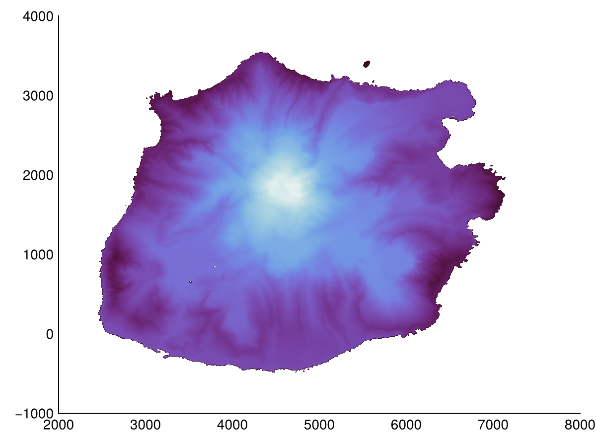
In these pages we will use the elevation model of Saba to showcase the different categories of operations that are available in Geomorphometry.jl. However, any DEM should work, most algorithms accept an AbstractMatrix{<:Real}. Note that you thus need to remove missing values from your DEM, which is ideally done by interpolation, but a quick coalesce.(dem, NaN32) will work too (but will cause NaN gaps in your output). Below are the steps to reproduce the example plots.
using Downloads

dtm_fn = abspath("saba.tif")
isfile(dtm_fn) || Downloads.download(
    "https://github.com/Deltares/Geomorphometry.jl/releases/download/v0.6.0/saba.tif",
    dtm_fn,
)
dsm_fn = abspath("saba_dsm.tif")
isfile(dsm_fn) || Downloads.download(
    "https://github.com/Deltares/Geomorphometry.jl/releases/download/v0.6.0/saba_dsm.tif",
    dsm_fn,
)
Details
You can download the data yourself from https://www.beeldmateriaal.nl/dataroom-caribisch-nederland, specifically the DTM and DSM. I've resampled them to a coarser resolution (from 0.5 m to 5 m), interpolated some nodata areas, and attached them to a Github release https://github.com/Deltares/Geomorphometry.jl/releases/tag/v0.6.0.
Visualization
Visualization is done using the hillshade, multihillshade, and pssm functions. The first two shade the terrain by using a single or multiple light source(s) respectively, while pssm is a slope map exaggerated for human perception.
heatmap(hillshade(dtm))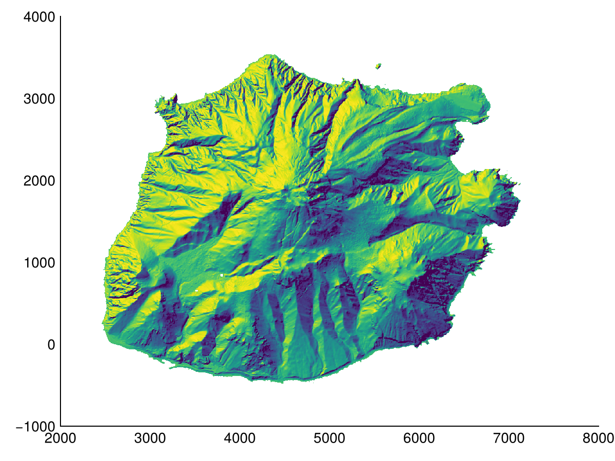
We can also overlay the pssm visualization on top of a colored aspect map.
f = heatmap(aspect(dtm); colormap=:curl)
heatmap!(pssm(dtm); colormap=Reverse(:greys), alpha=0.5)
f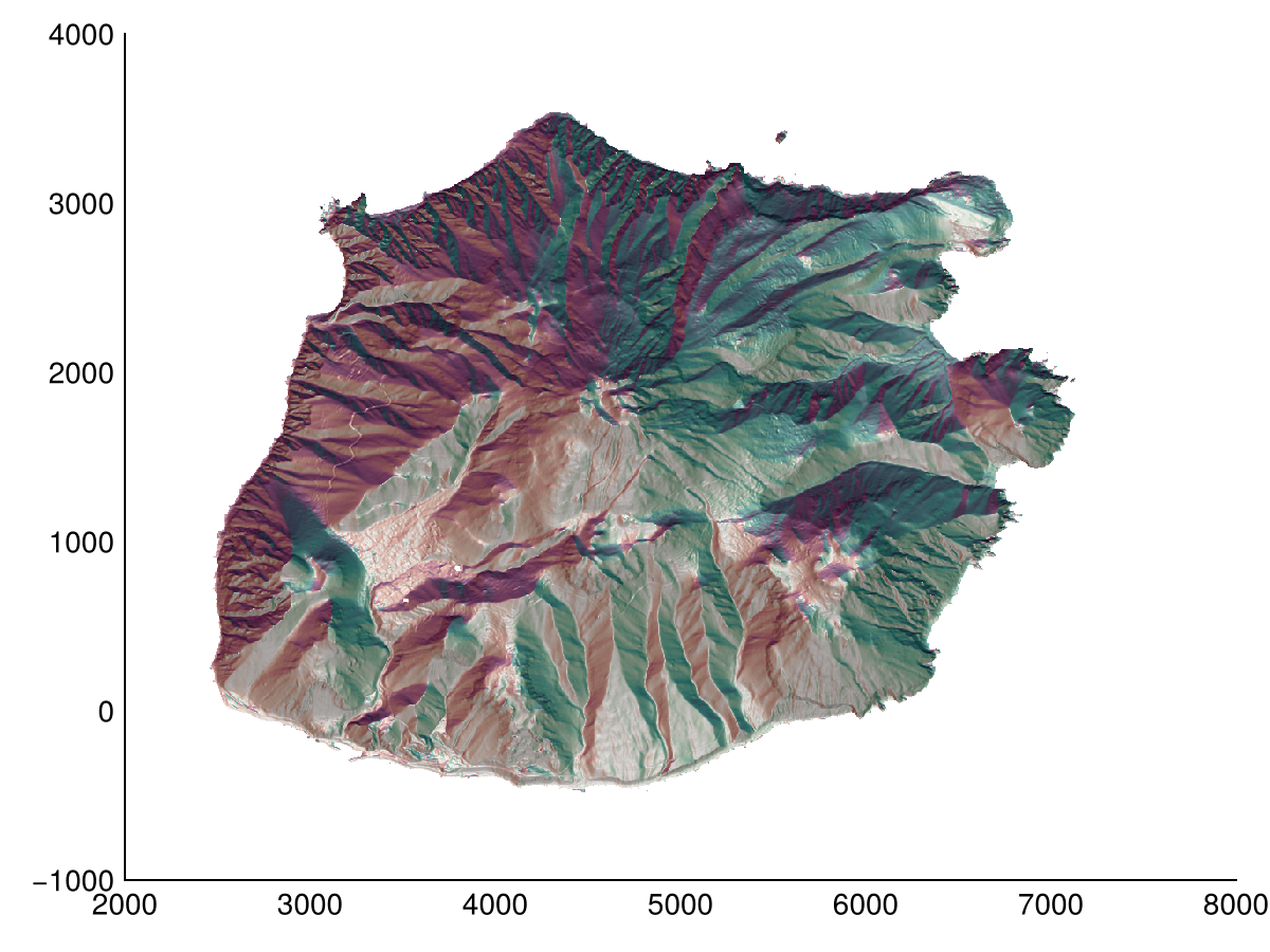
Derivatives
Common derivatives are implemented in Geomorphometry.jl. These include slope, aspect, and curvature. The latter is ill-defined, here we provide plan_curvature (also called projected contour curvature), profile_curvature (also called normal slope line curvature), and tangential_curvature (also called normal contour curvature). Note that functions here allow for a custom radius, as demonstrated for profile_curvature.
Slope
heatmap(slope(dtm; method=Horn()); colormap=:matter, colorrange=(0, 60))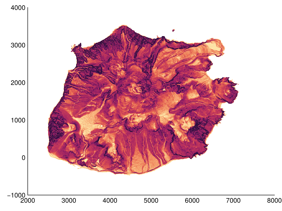
We can also determine the slope of the terrain along a specific direction.
heatmap(slope(dtm; method=Horn(), direction=0); colormap=:matter, colorrange=(-45, 45))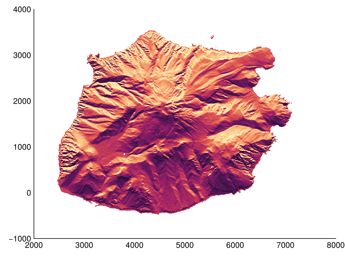
Aspect
heatmap(aspect(dtm; method=Horn()); colormap=:romaO)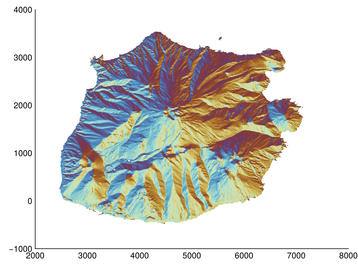
Curvature
heatmap(profile_curvature(dtm); colorrange=(-1,1), colormap=:tarn)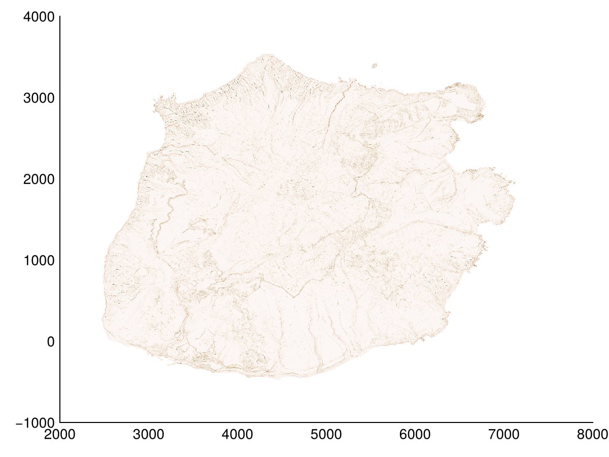
We can also determine the curvature of the terrain along a specific direction.
heatmap(laplacian(dtm, radius=1, direction=90); colorrange=(-1,1), colormap=:tarn)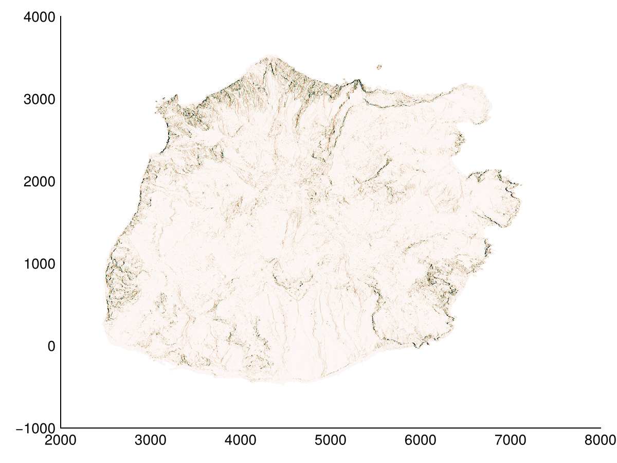
Relative position
There are several terrain descriptors that can be used to analyze the relative position of a point with respect to its neighbors. These include topographic_position_index, terrain_ruggedness_index, roughness_index_elevation, bathymetric_position_index, rugosity, roughness and percentile_elevation. Here we use bathymetric_position_index, but with a custom sized Window (from Stencils.jl). All these functions can be used with a custom window size.
heatmap(bathymetric_position_index(dtm, Geomorphometry.Annulus(5, 3)); colormap=:delta, colorrange=(-10,10))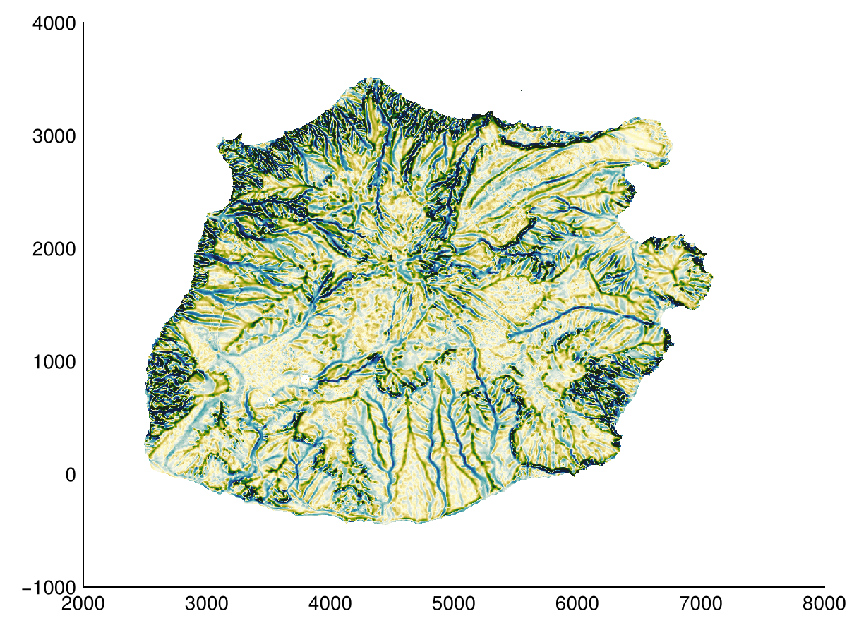
Horizon
Related to the relative position is the category related to the view (to a horizon) from any cell in a DEM. We have horizon_angle to compute the maximum horizon angle for a given number of directions, and sky_view_factor to compute fraction of the sky (hemisphere) visible from a cell. The same running-maximum test powers viewshed, the line-of-sight visibility map of a single observer cell, and total_viewshed, a normalized visibility index for every cell.
hor = horizon_angle(dtm)  # this produces a width,height,directions sized raster
heatmap(hor[:,:,1]; colormap=:curl, colorrange=(-90, 90))  # first direction (east) out of 16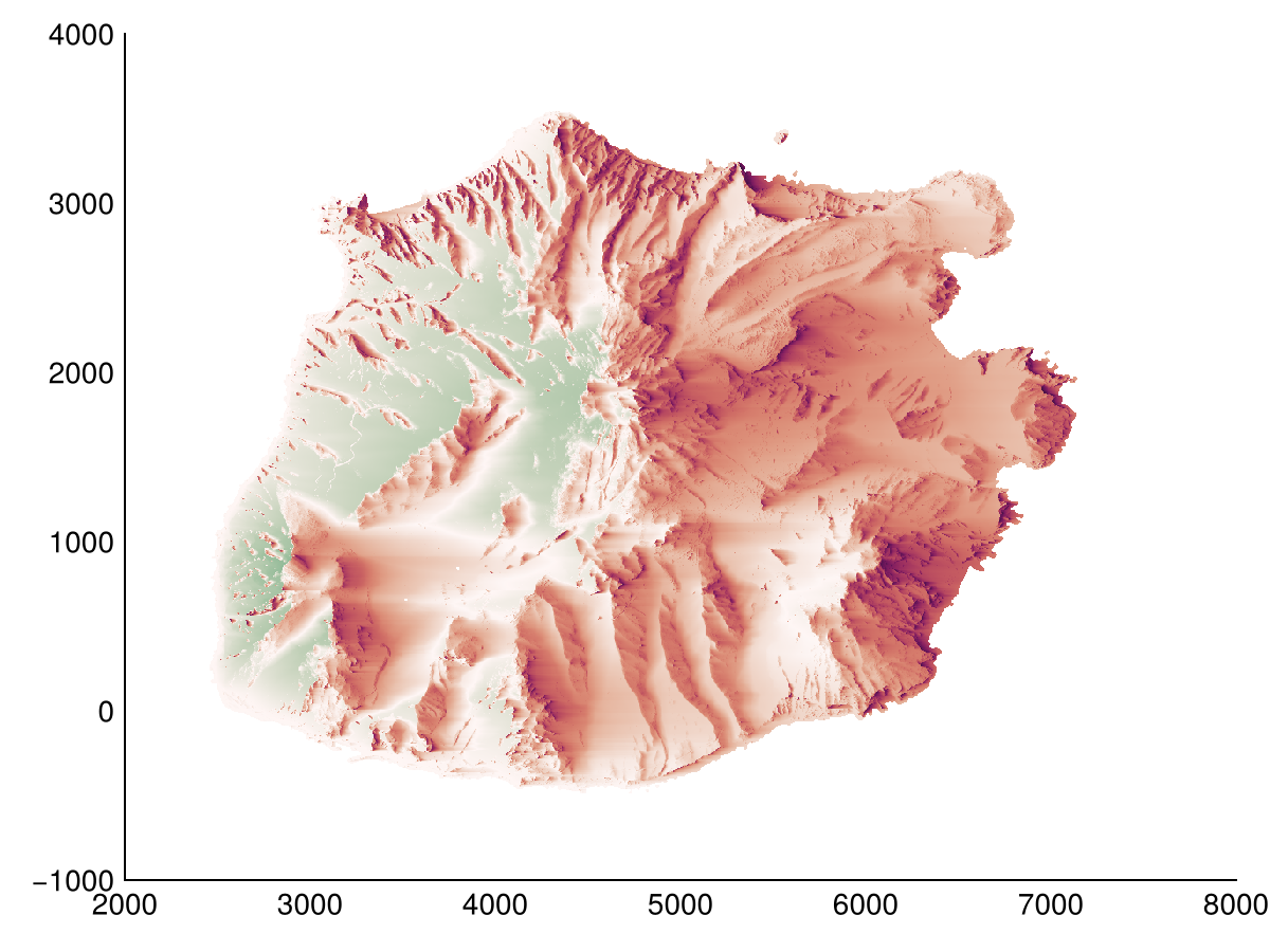
Landforms
The same lines of sight also classify the terrain itself. geomorphon reduces the view in eight directions to a ternary pattern of rising, flat and falling directions, and maps it onto one of ten Landform classes. The radius keyword sets the scale of the classification, while flatness sets how much relief a direction needs before it is no longer considered flat.
forms = geomorphon(dtm)
heatmap(forms; colormap=:tab10, colorrange=(0.5, 10.5), lowclip=:transparent)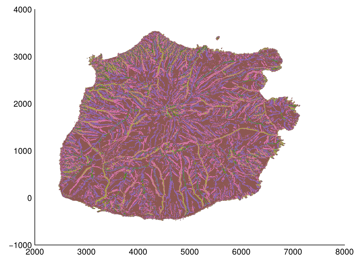
Hydrology
Hydrological operations are used to analyze the flow of water on the terrain. We provide filldepressions to fill depressions, depression_depth to calculate the depth of each depression (difference between filled dem and dem) and depression_volume that sums all depression depths. The major depression in the example is the caldera of the dormant volcano (Mount Scenery).
cdtm = copy(dtm)
cdtm[mask] .= -Inf  # Sea should be lower than terrain
fdtm = filldepressions(cdtm)
heatmap(fdtm)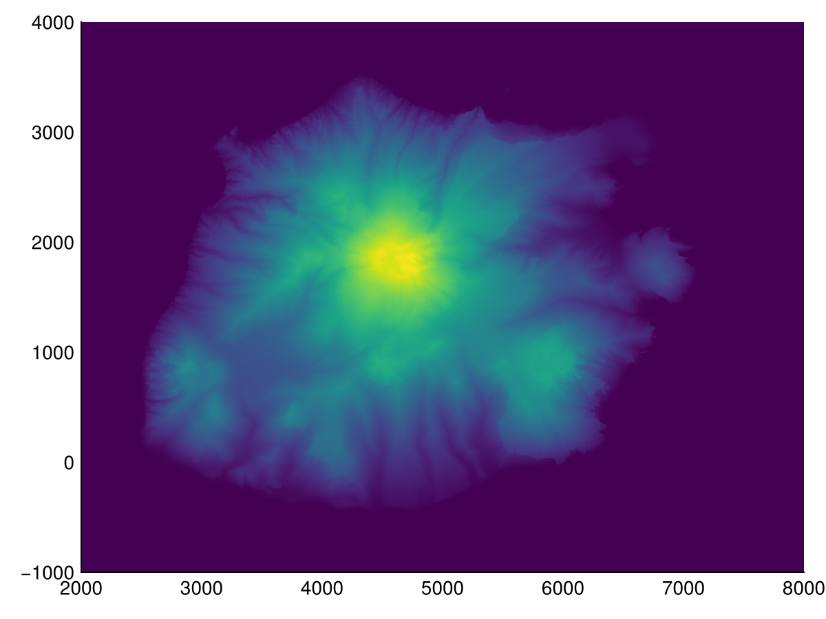
Filling the depressions in a DEM is not necessary to calculate the flow accumulation. Here we use flowaccumulation to do so, and it automatically carves out depressions. Note that the local drainage direction is also returned. By default the FD8 algorithm is used, but you can also use the D∞ or D8 algorithm by setting the method keyword argument to DInf() or D8().
WARNING
Most hydrology related methods iterate through all DEM cells, thus producing output for all DEM cells, including cells containing nodata values (e.g. NaN32, Inf). Here we manually hide these nodata areas for plotting.
acc, ldd = flowaccumulation(dtm; method=FD8(2))
acc[mask] .= NaN32  # ignore nodata areas for plotting
heatmap(log10.(acc); colormap=:rain)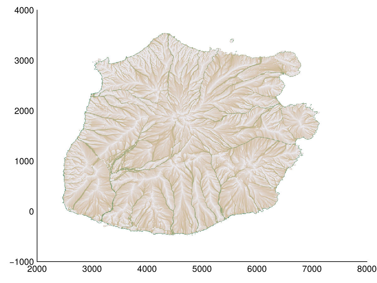
Combined with the previous analysis, we can calculate topographic_wetness_index, stream_power_index and drainage_potential indices. These indices are used to analyze the terrain's ability to accumulate water, the terrain's ability to store water respectively, and the ability to drain water respectively.
twi = topographic_wetness_index(dtm; method=FD8())
heatmap(twi; colormap=:tempo)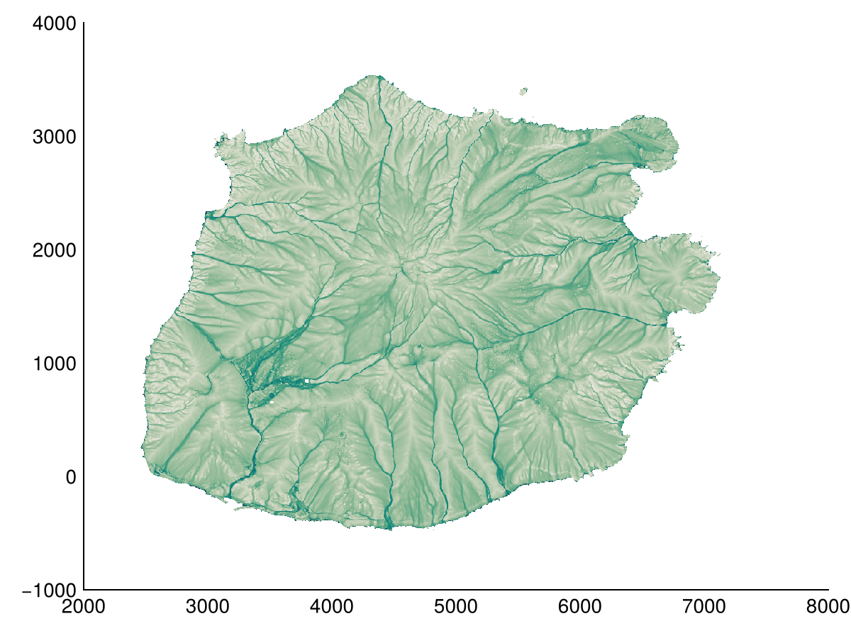
We can also calculate the Height Above Nearest Drainage (HAND) using the height_above_nearest_drainage function. This function requires a flow accumulation map to determine the stream network. Here we use a threshold based on the flow accumulation to define streams.
hand = height_above_nearest_drainage(dtm; threshold=1e3)
hand[mask] .= NaN32  # ignore nodata areas for plotting
heatmap(hand; colormap=:turbo)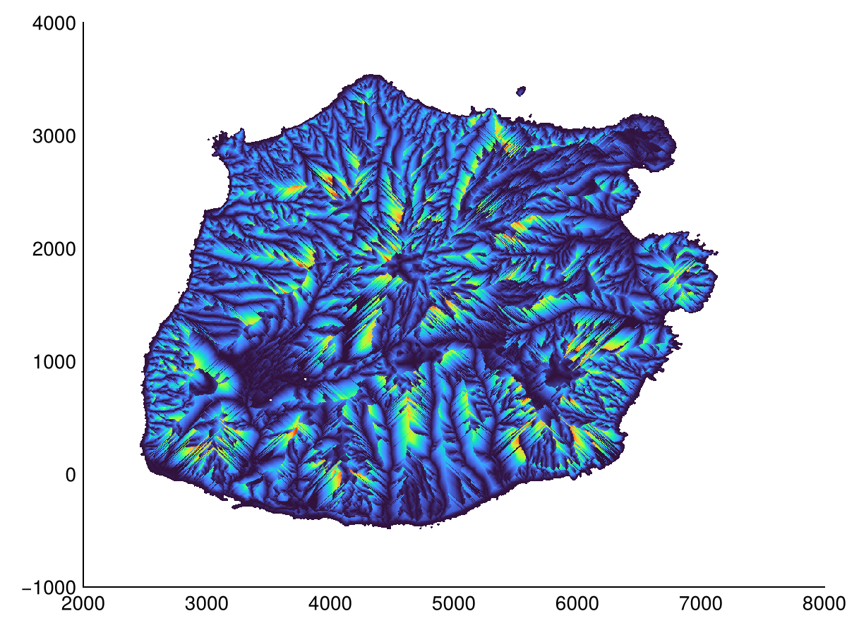
Terrain filters
While filters seem unrelated to the previously discussed methods, these are used to filter (rasterized) pointclouds i.e. surface models (DSM) to arrive at a terrain model (DTM). We provide progressive_morphological_filter, simple_morphological_filter, and skewness_balancing filters. Here we use the progressive_morphological_filter filter to remove elevations that do not pass the slope filter (normally vegetation and buildings).
B, flags = progressive_morphological_filter(dsm, ωₘ = 15.0, slope = 0.2, dhₘ = 5.0, dh₀ = 0.3)
A = copy(dsm)
A[A .> B] .= NaN32
heatmap(A)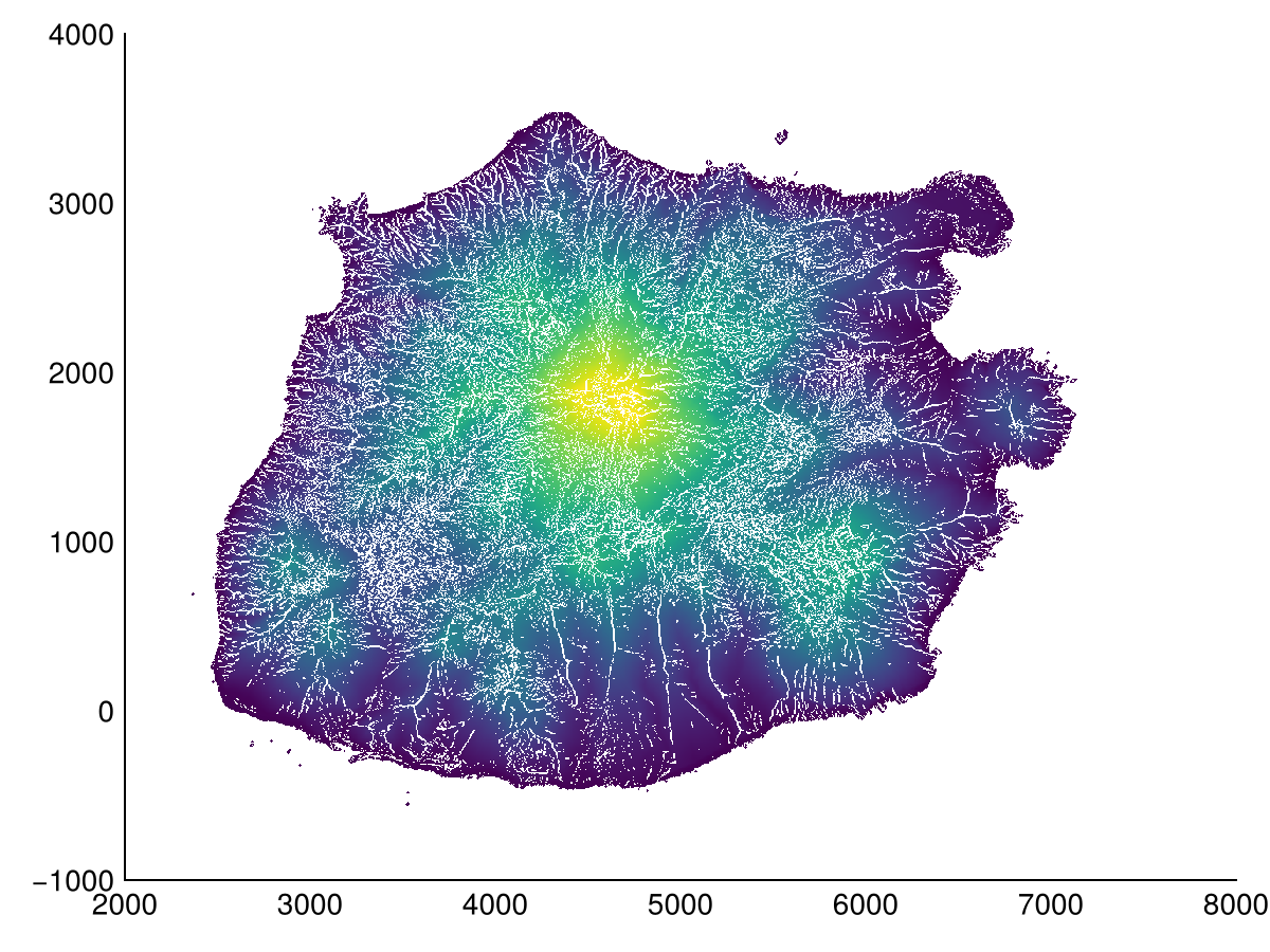
Cost distance
Finally there are so-called cost distance functions. Instead of calculating a distance in the Euclidean sense, these functions calculate the cost of moving from one point to another, given a spatial varying cost. We provide a single spread function with multiple methods. The function takes starting points, an initial cost, and a cost (friction) map.
Here we use the top of the volcano as the starting point, and the squared slope as the cost map. We compare the Tomlin method with the Eikonal and Eastman methods. Eastman requires a high number of iterations to converge (even at 25 it's not enough), and is thus slower.
tspread = spread(dtm .> 850, 0, slope(dtm).^2)
tspread[mask] .= NaN32  # ignore nodata areas for plotting
heatmap(tspread, colormap=:dense)