Centroid Voronoi Tesselation (CVT)

In principle, computing a centroid voronoi tesslation mesh from an existing mesh of convex cells is easy:

• Compute the centroids of the cells.

• Invert the face_node_connectivity index array.

• For every node, find the connected faces.

• Use the connected faces to find the centroids.

• Order the centroids around the vertex in a counter-clockwise manner.

Dealing with the mesh exterior (beyond which no centroids are located) is the tricky part.

For simplicity this example will only deal with (bare) numpy and scipy.sparse arrays. This example therefore also shows how to use these modules, should you not want to rely on more complex dependencies such as xugrid and xarray.

import matplotlib.pyplot as plt
import matplotlib.tri as mtri
import numpy as np
from matplotlib.collections import LineCollection, PolyCollection

From xugrid, we need only import the connectivity and voronoi modules. The functions in these modules depend only on numpy and scipy.sparse.

from xugrid.ugrid import connectivity, voronoi


def generate_disk(partitions: int, depth: int):
    """
    Generate a triangular mesh for the unit circle.

    Parameters
    ----------
    partitions: int
        Number of triangles around the origin.
    depth: int
        Number of "layers" of triangles around the origin.

    Returns
    -------
    vertices: np.ndarray of floats with shape ``(n_vertex, 2)``
    triangles: np.ndarray of integers with shape ``(n_triangle, 3)``
    """
    N = depth + 1
    n_per_level = partitions * np.arange(N)
    n_per_level[0] = 1

    delta_angle = (2 * np.pi) / np.repeat(n_per_level, n_per_level)
    index = np.repeat(np.insert(n_per_level.cumsum()[:-1], 0, 0), n_per_level)
    angles = delta_angle.cumsum()
    angles = angles - angles[index] + 0.5 * np.pi
    radii = np.repeat(np.linspace(0.0, 1.0, N), n_per_level)

    x = np.cos(angles) * radii
    y = np.sin(angles) * radii
    triang = mtri.Triangulation(x, y)
    return np.column_stack((x, y)), triang.triangles


def edge_plot(vertices, edge_nodes, ax, fill_value=-1, **kwargs):
    n_edge = len(edge_nodes)
    edge_coords = np.empty((n_edge, 2, 2), dtype=float)
    node_0 = edge_nodes[:, 0]
    node_1 = edge_nodes[:, 1]
    valid = (node_0 != fill_value) & (node_1 != fill_value)
    node_0 = node_0[valid]
    node_1 = node_1[valid]
    edge_coords[:, 0, 0] = vertices[node_0, 0]
    edge_coords[:, 0, 1] = vertices[node_0, 1]
    edge_coords[:, 1, 0] = vertices[node_1, 0]
    edge_coords[:, 1, 1] = vertices[node_1, 1]
    collection = LineCollection(edge_coords, **kwargs)
    primitive = ax.add_collection(collection)
    ax.autoscale()
    return primitive


def face_plot(vertices, face_nodes, ax, fill_value=-1, **kwargs):
    vertices = vertices[face_nodes]
    # Replace fill value; PolyCollection ignores NaN.
    vertices[face_nodes == fill_value] = np.nan
    collection = PolyCollection(vertices, **kwargs)
    primitive = ax.add_collection(collection)
    ax.autoscale()
    return primitive


def comparison_plot(
    vertices0,
    faces0,
    centroids0,
    vertices1,
    faces1,
):
    fig, (ax0, ax1, ax2) = plt.subplots(
        nrows=1,
        ncols=3,
        figsize=(15, 5),
        subplot_kw={"box_aspect": 1},
        sharey=True,
        sharex=True,
    )

    edges0, _ = connectivity.edge_connectivity(faces0, -1)
    edge_plot(vertices0, edges0, ax0, colors="black")
    ax0.scatter(*centroids0.T, color="red")
    ax0.scatter(*vertices0.T, color="black")

    edges1, _ = connectivity.edge_connectivity(faces1, -1)
    edge_plot(vertices0, edges0, ax1, colors="black")
    edge_plot(vertices1, edges1, ax1, colors="red")

    edge_plot(vertices1, edges1, ax2, colors="red")
    ax2.scatter(*vertices0.T, color="black")
    ax2.scatter(*centroids0.T, color="red")

    return fig

Let’s start by generating a simple unstructured mesh and use only its centroids to generate a voronoi tesselation.

Note: -1 functions as the fill value in this example.

vertices, faces = generate_disk(5, 2)
centroids = vertices[faces].mean(axis=1)

node_face_connectivity = connectivity.invert_dense_to_sparse(faces, -1)
voronoi_vertices, voronoi_faces, face_index = voronoi.voronoi_topology(
    node_face_connectivity,
    vertices,
    centroids,
    add_exterior=False,
    add_vertices=False,
)
voronoi_faces = connectivity.to_dense(voronoi_faces, -1)

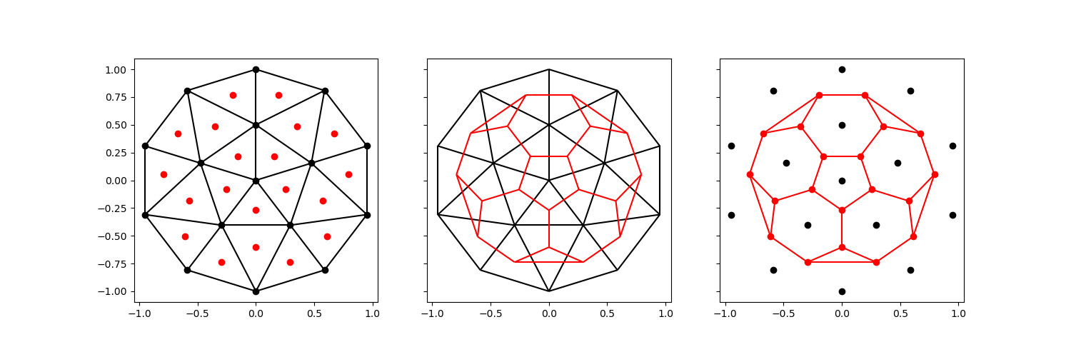
We can compare the two meshes:

• Left the original mesh, with centroids colored red

• The new mesh, overlaid on the original mesh.

• Right the new mesh, with its centroids – the original vertices – colored black.

comparison_plot(vertices, faces, centroids, voronoi_vertices, voronoi_faces)

<Figure size 1500x500 with 3 Axes>

It should be clear that the new voronoi mesh is not space filling: since it uses only the centroids, we do not preserve the exterior.

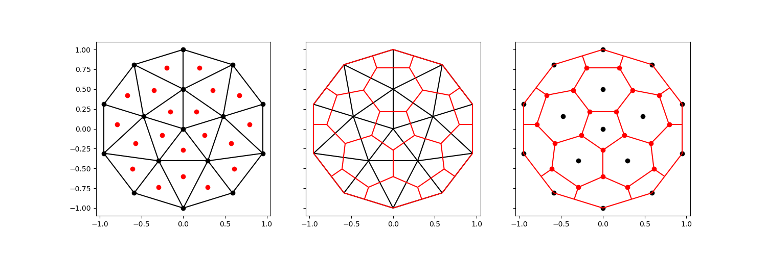
The voronoi_topology is capable of preserving the exterior exactly, but this requires more topological information.

edge_node_connectivity, face_edge_connectivity = connectivity.edge_connectivity(
    faces, -1
)
edge_face_connectivity = connectivity.invert_dense(face_edge_connectivity, -1)
voronoi_vertices, voronoi_faces, face_index = voronoi.voronoi_topology(
    node_face_connectivity,
    vertices,
    centroids,
    edge_face_connectivity=edge_face_connectivity,
    edge_node_connectivity=edge_node_connectivity,
    fill_value=-1,
    add_exterior=True,
    add_vertices=True,
)
voronoi_faces = connectivity.to_dense(voronoi_faces, -1)

comparison_plot(vertices, faces, centroids, voronoi_vertices, voronoi_faces)

<Figure size 1500x500 with 3 Axes>

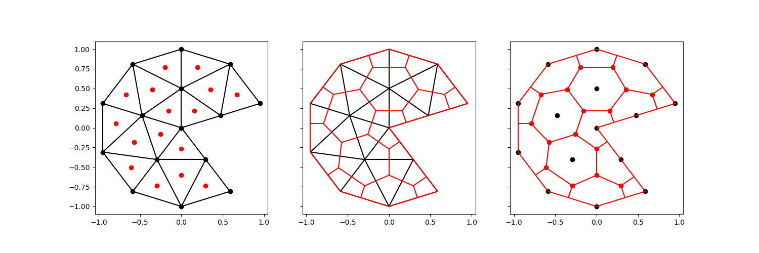
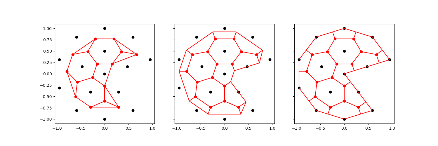
A potential downside of including the full exterior only becomes clear when we apply it to a mesh with a more complex exterior.

Let’s take the circular mesh above, and remove a chunk.

vertices, faces = generate_disk(5, 2)
centroids = vertices[faces].mean(axis=1)
dx, dy = centroids.T
angle = np.arctan2(dy, dx)
new = faces[(angle < -0.87) | (angle > 0.27)]
vertices = vertices[np.unique(new.ravel())]
faces = connectivity.renumber(new)
centroids = vertices[faces].mean(axis=1)

node_face_connectivity = connectivity.invert_dense_to_sparse(faces, -1)
edge_node_connectivity, face_edge_connectivity = connectivity.edge_connectivity(
    faces, -1
)
edge_face_connectivity = connectivity.invert_dense(face_edge_connectivity, -1)
voronoi_vertices, voronoi_faces, face_index = voronoi.voronoi_topology(
    node_face_connectivity,
    vertices,
    centroids,
    edge_face_connectivity=edge_face_connectivity,
    edge_node_connectivity=edge_node_connectivity,
    fill_value=-1,
    add_exterior=True,
    add_vertices=True,
)
voronoi_faces = connectivity.to_dense(voronoi_faces, -1)

comparison_plot(vertices, faces, centroids, voronoi_vertices, voronoi_faces)

<Figure size 1500x500 with 3 Axes>

The voronoi cell in the center of the disk has now become concave. This will generally render the mesh unsuitable for finite volume or control volume finite difference simulations.

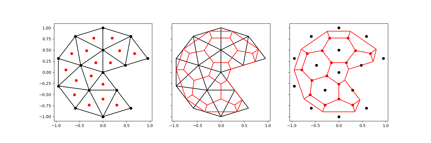
We can circumvent this difficulty entirely, by ignoring the exterior vertices of the original mesh altogether. We still add an orthogonal projection of every centroid to exterior edges.

node_face_connectivity = connectivity.invert_dense_to_sparse(faces, -1)
edge_node_connectivity, face_edge_connectivity = connectivity.edge_connectivity(
    faces, -1
)
edge_face_connectivity = connectivity.invert_dense(face_edge_connectivity, -1)
voronoi_vertices, voronoi_faces, face_index = voronoi.voronoi_topology(
    node_face_connectivity,
    vertices,
    centroids,
    edge_face_connectivity=edge_face_connectivity,
    edge_node_connectivity=edge_node_connectivity,
    fill_value=-1,
    add_exterior=True,
    add_vertices=False,
)
voronoi_faces = connectivity.to_dense(voronoi_faces, -1)

comparison_plot(vertices, faces, centroids, voronoi_vertices, voronoi_faces)

<Figure size 1500x500 with 3 Axes>

This will (obviously) result in a mesh that does not preserve the exterior exactly.

These are the three options, side by side:

nodes0, faces0, face_index0 = voronoi.voronoi_topology(
    node_face_connectivity,
    vertices,
    centroids,
)
faces0 = connectivity.to_dense(faces0, -1)
edges0, _ = connectivity.edge_connectivity(faces0, -1)

nodes1, faces1, face_index1 = voronoi.voronoi_topology(
    node_face_connectivity,
    vertices,
    centroids,
    edge_face_connectivity=edge_face_connectivity,
    edge_node_connectivity=edge_node_connectivity,
    fill_value=-1,
    add_exterior=True,
    add_vertices=False,
)
faces1 = connectivity.to_dense(faces1, -1)
edges1, _ = connectivity.edge_connectivity(faces1, -1)

nodes2, faces2, _ = voronoi.voronoi_topology(
    node_face_connectivity,
    vertices,
    centroids,
    edge_face_connectivity=edge_face_connectivity,
    edge_node_connectivity=edge_node_connectivity,
    fill_value=-1,
    add_exterior=True,
    add_vertices=True,
)
faces2 = connectivity.to_dense(faces2, -1)
edges2, _ = connectivity.edge_connectivity(faces2, -1)


fig, axes = plt.subplots(
    nrows=1,
    ncols=3,
    figsize=(15, 5),
    subplot_kw={"box_aspect": 1},
    sharey=True,
    sharex=True,
)
all_edges = [edges0, edges1, edges2]
all_nodes = [nodes0, nodes1, nodes2]
for ax, e, v in zip(axes, all_edges, all_nodes):
    edge_plot(v, e, ax, colors="red")
    ax.scatter(*centroids.T, color="red")
    ax.scatter(*vertices.T, color="black")

Plotting

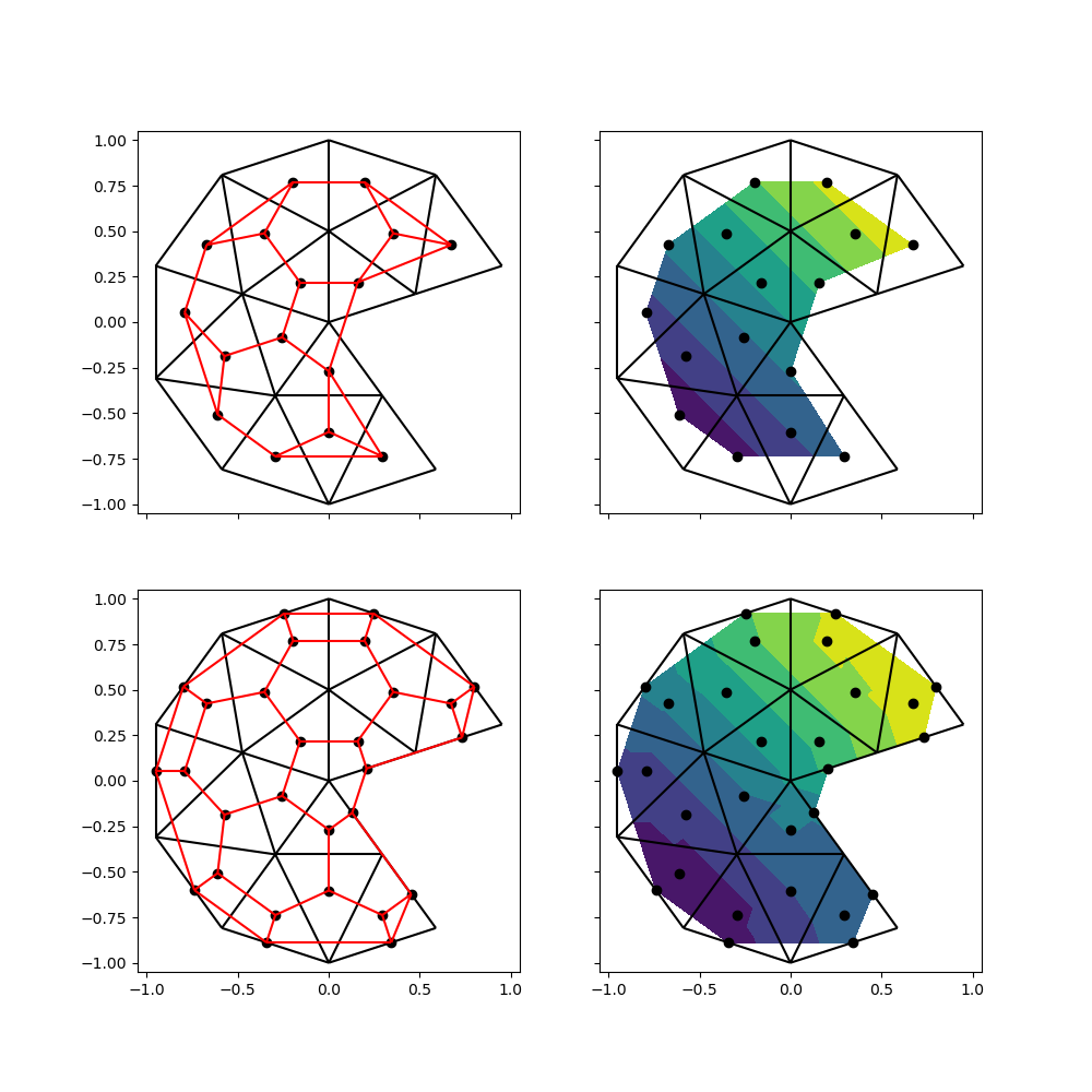
One of the uses of a voronoi tesselation is to visualize data that is located on the faces. This is once again relevant for finite volume or finite difference simulations; finite element simulation data is located on the nodes of the mesh.

For the sake of this example, let’s assume we have data (e.g. pressure) that varies linearly from the lower left to the upper right.

data = centroids[:, 0] + centroids[:, 1]

Before we can send the data of an unstructured mesh off to a plotting library such as matplotlib, we’ll generally need to triangulate the mesh. We can directly use the first two options, since the generated voronoi vertices correspond directly to a cell face. This is not the case for the third option, since it includes some vertices of the original mesh, which are connected to two faces.

triangles0, face_triangles0 = connectivity.triangulate(faces0, -1)
triangulation0 = mtri.Triangulation(nodes0[:, 0], nodes0[:, 1], triangles0)

triangles1, face_triangles1 = connectivity.triangulate(faces1, -1)
triangulation1 = mtri.Triangulation(nodes1[:, 0], nodes1[:, 1], triangles1)


fig, ((ax0, ax1), (ax2, ax3)) = plt.subplots(
    nrows=2,
    ncols=2,
    figsize=(10, 10),
    subplot_kw={"box_aspect": 1},
    sharey=True,
    sharex=True,
)

edge_plot(vertices, edge_node_connectivity, ax0, colors="black")
ax0.scatter(*nodes0.T, color="black")
edge_plot(nodes0, edges0, ax0, colors="red")

ax1.tricontourf(triangulation0, data[face_index0])
ax1.scatter(*nodes0.T, color="black")
edge_plot(vertices, edge_node_connectivity, ax1, colors="black")

edge_plot(vertices, edge_node_connectivity, ax2, colors="black")
ax2.scatter(*nodes1.T, color="black")
edge_plot(nodes1, edges1, ax2, colors="red")

ax3.tricontourf(triangulation1, data[face_index1])
ax3.scatter(*nodes1.T, color="black")
edge_plot(vertices, edge_node_connectivity, ax3, colors="black")

ax0.set_xlim(-1.05, 1.05)
ax0.set_ylim(-1.05, 1.05)

(-1.05, 1.05)

While the second option fills a greater proportion than the first option – which is confined to the area between the centroids – it’s clear this approach results in artifacts in the exterior voronoi cells.

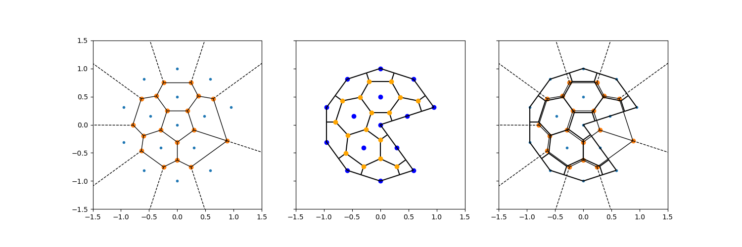
Infinite rays

When only vertices are considered, the voronoi edges between the most outward vertices are unbounded: they extend into infinity (the dotted lines in the plots below). These can be intersected with the mesh exterior.

The figure shows:

• The voronoi tesselation (including infinite edges) made by scipy.spatial.Voronoi.

• The voronoi tesslation produced by the voronoi_topology function in xugrid, along with original vertices in blue, and the original centroids in orange.

• Both of them, overlaid in the same plot.

from scipy.spatial import Voronoi, voronoi_plot_2d

vor = Voronoi(vertices)

fig, (ax0, ax1, ax2) = plt.subplots(
    figsize=(15, 5),
    nrows=1,
    ncols=3,
    subplot_kw={"box_aspect": 1},
    sharex=True,
    sharey=True,
)

voronoi_plot_2d(vor, ax=ax0)

edge_plot(nodes2, edges2, ax1, colors="black")
ax1.scatter(*vertices.T, color="blue")
ax1.scatter(*centroids.T, color="orange", zorder=3)

voronoi_plot_2d(vor, ax=ax2)
edge_plot(nodes2, edges2, ax2, colors="black")

ax0.set_xlim(-1.5, 1.5)
ax0.set_ylim(-1.5, 1.5)

(-1.5, 1.5)