Delineation of (sub)basins#

Here we assume that flow directions are known. We read the flow direction raster data, including meta-data, using rasterio and parse it to a pyflwdir FlwDirRaster object, see earlier examples for more background.

[1]:

# import pyflwdir, some dependencies
import geopandas as gpd
import numpy as np
import rasterio
from matplotlib import cm

# local convenience methods (see utils.py script in notebooks folder)
from utils import quickplot, vectorize

import pyflwdir

# read and parse data
with rasterio.open("rhine_d8.tif", "r") as src:
    flwdir = src.read(1)
    crs = src.crs
    flw = pyflwdir.from_array(
        flwdir,
        ftype="d8",
        transform=src.transform,
        latlon=crs.is_geographic,
        cache=True,
    )

Outlet based (sub)basins#

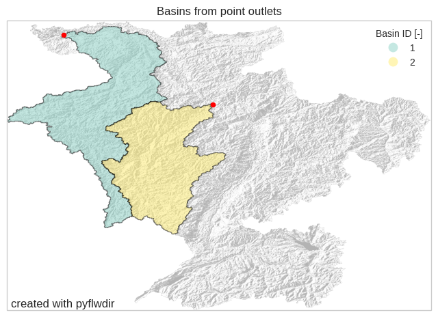
By default, this method uses pits in the flow-direction raster as basin outlets. If outlet locations are provided, it uses those instead. You can also pass a streams argument to snap outlet locations to the nearest downstream stream cell. This uses the snap() method under the hood. Here, streams are defined using a minimum Strahler stream order of 4.

[2]:

# define output locations
x, y = np.array([4.67916667, 7.60416667]), np.array([51.72083333, 50.3625])
gdf_out = gpd.GeoSeries(gpd.points_from_xy(x, y, crs=4326))
# delineate subbasins
subbasins = flw.basins(xy=(x, y), streams=flw.stream_order() >= 4)
# vectorize subbasins using the vectorize convenience method from utils.py
gdf_bas = vectorize(subbasins.astype(np.int32), 0, flw.transform, name="basin")
gdf_bas.head()

[2]:

	geometry	basin
0	POLYGON ((5.55833 51.89167, 5.55833 51.88333, ...	1
1	POLYGON ((6.45833 50.425, 6.45833 50.41667, 6....	2

[3]:

# plot
# keyword arguments passed to GeoDataFrame.plot()

gpd_plot_kwds = {
    "column": "basin",
    "cmap": cm.Set3,
    "legend": True,
    "categorical": True,
    "legend_kwds": {"title": "Basin ID [-]"},
    "alpha": 0.5,
    "edgecolor": "black",
    "linewidth": 0.8,
}
points = (gdf_out, {"color": "red", "markersize": 20})
bas = (gdf_bas, gpd_plot_kwds)
# plot using quickplot convenience method from utils.py
ax = quickplot([bas, points], title="Basins from point outlets", filename="flw_basins")

River confluence subbasins#

The default subbasins() method creates subbasins at all confluences of the river network.

[4]:

# calculate subbasins for all stream segments with a minimum upstream area of 100 km2
mask = flw.upstream_area(unit="km2") >= 100
subbas, idxs_out = flw.subbasins(riv_mask=mask)
# transform map and point locations to GeoDataFrames
gdf_subbas = vectorize(subbas.astype(np.int32), 0, flw.transform, name="basin")
gdf_out = gpd.GeoSeries(gpd.points_from_xy(*flw.xy(idxs_out), crs=4326))
# plot
gpd_plot_kwds = {
    "column": "basin",
    "cmap": cm.Set3,
    "edgecolor": "black",
    "alpha": 0.6,
    "linewidth": 0.5,
}
bas = (gdf_subbas, gpd_plot_kwds)
points = (gdf_out, {"color": "k", "markersize": 10})
title = "Subbasins for all stream segments with a minimum upstream area of 100 km2"
ax = quickplot([bas, points], title=title, filename="flw_subbasins")

Stream order subbasins#

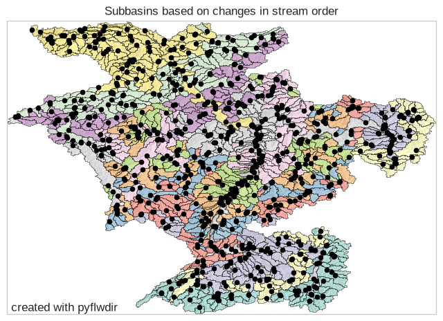
The subbasins_streamorder() method creates subbasins at all confluences where a lower order stream segments enters a higher order segment. An optional mask of valid cells can be added to constrain the selection of outlets to rivers within the mask based on e.g. a minimum upstream area threshold.

[5]:

# calculate stream-order subbasins for a river network with a minimum upstream area of 100 km2
mask = flw.upstream_area(unit="km2") >= 100
subbas, idxs_out = flw.subbasins_streamorder(min_sto=0, mask=mask)
# transform map and point locations to GeoDataFrames
gdf_subbas = vectorize(subbas.astype(np.int32), 0, flw.transform, name="basin")
gdf_out = gpd.GeoSeries(gpd.points_from_xy(*flw.xy(idxs_out), crs=4326))
# plot
gpd_plot_kwds = {
    "column": "basin",
    "cmap": cm.Set3,
    "edgecolor": "black",
    "alpha": 0.6,
    "linewidth": 0.5,
}
bas = (gdf_subbas, gpd_plot_kwds)
points = (gdf_out, {"color": "k", "markersize": 20})
title = "Subbasins based on changes in stream order"
ax = quickplot([bas, points], title=title, filename="flw_subbasins_streamorder")
gdf_subbas.to_file("flw_subbasins.gpkg", driver="GPKG")

Pfafstetter subbasins#

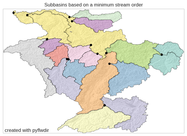
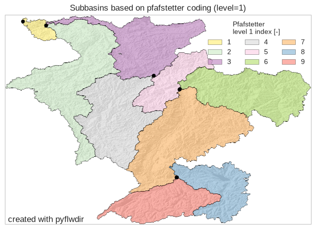
The subbasins_pfafstetter() method creates subbasins using the hierarchical Pfafstetter coding system. The codes encode topological information, making it easy to determine whether one subbasin is downstream of another. At each level, the four largest subbasins receive even numbers, and the five largest interbasins receive odd numbers. Set depth to choose the number of levels: depth=1 produces 9 subbasin/interbasin units in total, while depth=2 produces 81. If uparea is not provided, the method calculates upstream area for each cell.

[6]:

# get the first-level Pfafstetter subbasins
pfafbas1, idxs_out = flw.subbasins_pfafstetter(depth=1)
# vectorize raster to obtain polygons
gdf_pfaf1 = vectorize(pfafbas1.astype(np.int32), 0, flw.transform, name="pfaf")
gdf_out = gpd.GeoSeries(gpd.points_from_xy(*flw.xy(idxs_out), crs=4326))
gdf_pfaf1.head()

[6]:

	geometry	pfaf
0	POLYGON ((4.10833 51.925, 4.10833 51.91667, 4....	1
1	POLYGON ((5.88333 52.00833, 5.88333 51.99167, ...	3
2	POLYGON ((8.95 51.075, 8.95 51.06667, 8.93333 ...	5
3	POLYGON ((8.96667 50.61667, 8.96667 50.60833, ...	6
4	POLYGON ((5.55833 51.89167, 5.55833 51.88333, ...	2

[7]:

# plot
gpd_plot_kwds = {
    "column": "pfaf",
    "cmap": cm.Set3_r,
    "legend": True,
    "categorical": True,
    "legend_kwds": {"title": "Pfafstetter \nlevel 1 index [-]", "ncol": 3},
    "alpha": 0.6,
    "edgecolor": "black",
    "linewidth": 0.4,
}

points = (gdf_out, {"color": "k", "markersize": 20})
bas = (gdf_pfaf1, gpd_plot_kwds)
title = "Subbasins based on pfafstetter coding (level=1)"
ax = quickplot([bas, points], title=title, filename="flw_pfafbas1")

[8]:

# create a second Pfafstetter layer with a minimum subbasin area of 5000 km2
pfafbas2, idxs_out = flw.subbasins_pfafstetter(depth=2, upa_min=5000)
gdf_pfaf2 = vectorize(pfafbas2.astype(np.int32), 0, flw.transform, name="pfaf2")
gdf_out = gpd.GeoSeries(gpd.points_from_xy(*flw.xy(idxs_out), crs=4326))
gdf_pfaf2["pfaf"] = gdf_pfaf2["pfaf2"] // 10
gdf_pfaf2.head()

[8]:

	geometry	pfaf2	pfaf
0	POLYGON ((5.88333 52.00833, 5.88333 51.99167, ...	31	3
1	POLYGON ((7.325 51.975, 7.325 51.95, 7.30833 5...	32	3
2	POLYGON ((6.58333 51.63333, 6.58333 51.625, 6....	33	3
3	POLYGON ((4.10833 51.925, 4.10833 51.91667, 4....	11	1
4	POLYGON ((7.2 51.63333, 7.2 51.625, 7.16667 51...	34	3

[9]:

# plot
bas = (gdf_pfaf2, gpd_plot_kwds)
points = (gdf_out, {"color": "k", "markersize": 20})
title = "Subbasins based on pfafstetter coding (level=2)"
ax = quickplot([bas, points], title=title, filename="flw_pfafbas2")

Minimal area based subbasins#

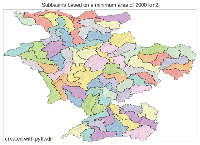
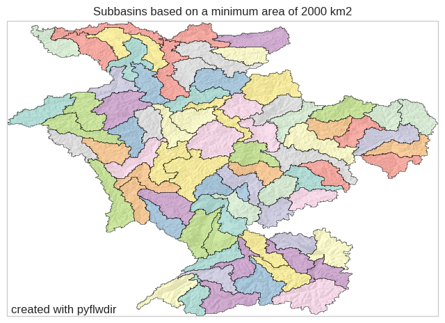
The subbasins_area() method creates subbasins with a minimum area of area_min. Moving upstream from the basin outlets, it starts a new subbasin at each tributary whose contributing area exceeds area_min. It starts a new interbasin when that interbasin’s area exceeds the same threshold.

[10]:

# calculate subbasins with a minimum area of 2000 km2
min_area = 2000
subbas, idxs_out = flw.subbasins_area(min_area)
# transform map and point locations to GeoDataFrames
gdf_subbas = vectorize(subbas.astype(np.int32), 0, flw.transform, name="basin")
# randomize index for visualization
basids = gdf_subbas["basin"].values
gdf_subbas["color"] = np.random.choice(basids, size=basids.size, replace=False)
# plot
gpd_plot_kwds = {
    "column": "color",
    "cmap": cm.Set3,
    "edgecolor": "black",
    "alpha": 0.6,
    "linewidth": 0.5,
}
bas = (gdf_subbas, gpd_plot_kwds)
title = f"Subbasins based on a minimum area of {min_area} km2"
ax = quickplot([bas], title=title, filename="flw_subbasins_area")