Spatial indexing of 1D networks and linear geometry#

This example demonstrates how to use the numba_celltree package to index 1D grids. The package provides a EdgeCellTree class that constructs a cell tree for 1D networks and linear geometries. The package currently supports the following operations:

Locating points
Locating line segments

This example provides an introduction to searching a cell tree for each of these.

We’ll start by importing the required packages with matplotlib for plotting.

import os

import matplotlib.pyplot as plt
import numpy as np
from matplotlib.collections import LineCollection

os.environ["NUMBA_DISABLE_JIT"] = "1"  # small examples, avoid JIT overhead
from numba_celltree import EdgeCellTree2d, demo  # noqa E402

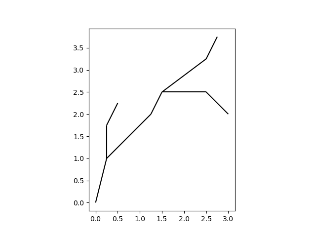
Let’s start with a simple 1D network.

vertices, edges = demo.example_1d_network()

node_x = vertices.T[0]
node_y = vertices.T[1]

fig, ax = plt.subplots()
demo.plot_edges(node_x, node_y, edges, ax, color="black")

Locating points#

We’ll build a cell tree first, then look for some points.

tree = EdgeCellTree2d(vertices, edges)
points = np.array(
    [
        [0.25, 1.5],
        [0.75, 1.5],
        [2.0, 1.5],  # This one is outside the grid
    ]
)
i = tree.locate_points(points)
i

array([ 7,  1, -1])

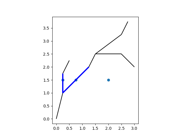
This returns the indices of the edges that contain each point, with -1 indicating points outside the network. We’ll have to filter those out first. Let’s plot them:

ii = i[i != -1]

fig, ax = plt.subplots()
ax.scatter(*points.transpose())
demo.plot_edges(node_x, node_y, edges, ax, color="black")
demo.plot_edges(node_x, node_y, edges[ii], ax, color="blue", linewidth=3)

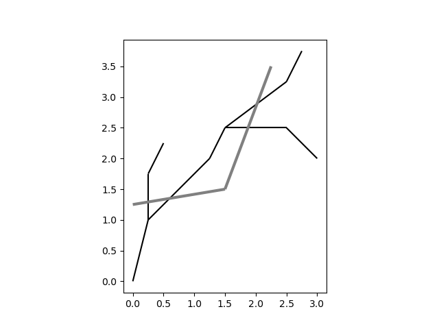
Locating line segments#

Let’s locate some line segments on the grid. We’ll start off with creating some line segments.

segments = np.array(
    [
        [[0.0, 1.25], [1.5, 1.5]],
        [[1.5, 1.5], [2.25, 3.5]],
    ]
)

fig, ax = plt.subplots()
demo.plot_edges(node_x, node_y, edges, ax, color="black")
ax.add_collection(LineCollection(segments, color="gray", linewidth=3))

<matplotlib.collections.LineCollection object at 0x7f33df11b830>

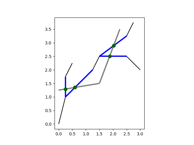
Let’s now intersect these line segments with the edges in the network.

segment_index, tree_edge_index, xy_intersection = tree.intersect_edges(segments)
xy_intersection

array([[0.6       , 1.35      ],
       [0.25      , 1.29166667],
       [2.02173913, 2.89130435],
       [1.875     , 2.5       ]])

The intersect_edges method returns three arrays: which input segments intersect with the network, which network edges they intersect with, and the coordinates of each intersection point.

Let’s plot the results:

fig, ax = plt.subplots()
demo.plot_edges(node_x, node_y, edges, ax, color="black")
demo.plot_edges(node_x, node_y, edges[tree_edge_index], ax, color="blue", linewidth=3)
ax.add_collection(LineCollection(segments, color="gray", linewidth=3))
ax.scatter(*xy_intersection.transpose(), s=60, color="darkgreen", zorder=2.5)

<matplotlib.collections.PathCollection object at 0x7f33df11ba70>

Total running time of the script: (0 minutes 0.219 seconds)

Gallery generated by Sphinx-Gallery

Spatial indexing of 1D networks and linear geometry#

Locating points#

Locating line segments#

This Page