Spatial indexing

The goal of a cell tree is to quickly locate cells of an unstructured mesh. Unstructured meshes are challenging in this regard: for a given point, we cannot simply compute a row and column number as we would for structured data such as rasters. The most straightforward procedure is checking every single cell, until we find the cell which contains the point we’re looking for. This is clearly not efficient.

A cell tree is bounding volume hierarchy (BVH) which may be used as a spatial index. A spatial index is a data structure to search a spatial object efficiently, without exhaustively checking every cell. The implementation in numba_celltree provides four ways to search the tree:

• Locating single points

• Locating bounding boxes

• Locating convex polygons (e.g. cells of another mesh)

• Locating line segments

This example provides an introduction to searching a cell tree for each of these.

We’ll start by importing the required packages with matplotlib for plotting.

import os

import matplotlib.pyplot as plt
import numpy as np
from matplotlib.collections import LineCollection

os.environ["NUMBA_DISABLE_JIT"] = "1"  # small examples, avoid JIT overhead
from numba_celltree import CellTree2d, demo  # noqa E402

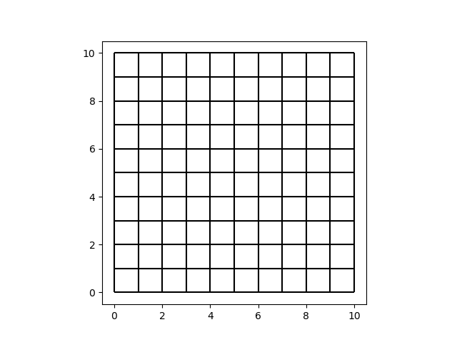
Let’s start with a rectangular mesh:

nx = ny = 10
x = y = np.linspace(0.0, 10.0, nx + 1)
vertices = np.array(np.meshgrid(x, y, indexing="ij")).reshape(2, -1).T
a = np.add.outer(np.arange(nx), nx * np.arange(ny)) + np.arange(ny)
faces = np.array([a, a + 1, a + nx + 2, a + nx + 1]).reshape(4, -1).T

Determine the edges of the cells, and plot them.

node_x, node_y = vertices.transpose()
edges = demo.edges(faces, -1)

fig, ax = plt.subplots()
demo.plot_edges(node_x, node_y, edges, ax, color="black")

Locating points

We’ll build a cell tree first, then look for some points.

tree = CellTree2d(vertices, faces, -1)
points = np.array(
    [
        [-5.0, 1.0],
        [4.5, 2.5],
        [6.5, 4.5],
    ]
)
i = tree.locate_points(points)
i

array([-1, 24, 46])

These numbers are the cell numbers in which we can find the points.

A value of -1 means that a point is not located in any cell.

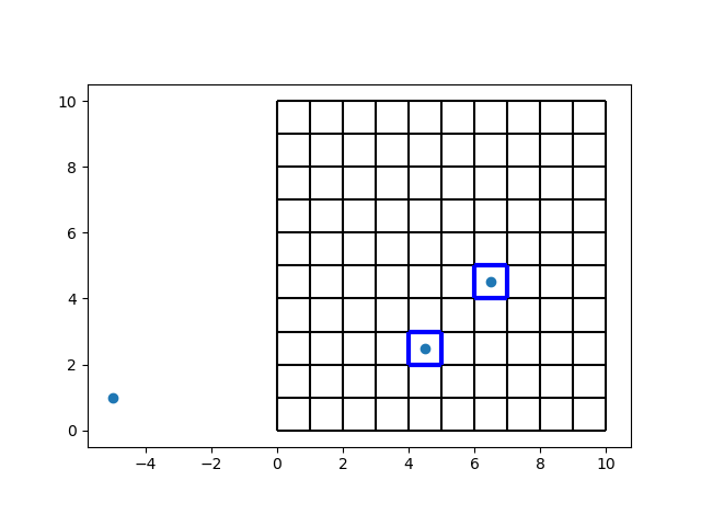
Let’s get rid of the -1 values, and take a look which cells have been found. We’ll color the found cells blue, and we’ll draw the nodes to compare.

i = i[i != -1]

fig, ax = plt.subplots()
ax.scatter(*points.transpose())
demo.plot_edges(node_x, node_y, edges, ax, color="black")
demo.plot_edges(node_x, node_y, demo.edges(faces[i], -1), ax, color="blue", linewidth=3)

Now let’s try a more exotic example.

vertices, faces = demo.generate_disk(5, 5)
vertices += 1.0
vertices *= 5.0
node_x, node_y = vertices.transpose()
edges = demo.edges(faces, -1)

fig, ax = plt.subplots()
demo.plot_edges(node_x, node_y, edges, ax, color="black")

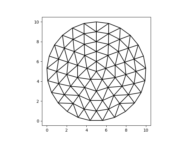
There are certainly no rows or columns to speak of!

Let’s build a new tree, and look for the same points as before.

tree = CellTree2d(vertices, faces, -1)
i = tree.locate_points(points)
i = i[i != -1]

fig, ax = plt.subplots()
ax.scatter(*points.transpose())
demo.plot_edges(node_x, node_y, edges, ax, color="black")
demo.plot_edges(node_x, node_y, demo.edges(faces[i], -1), ax, color="blue", linewidth=3)

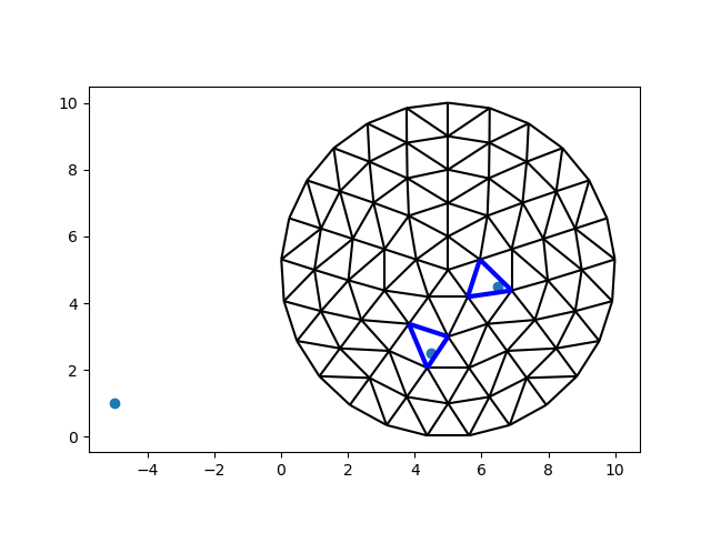
It should be clear by now that a point may only fall into a single cell. A point may also be out of bounds. If a cell falls exactly on an edge, one of the two neighbors will be chosen arbitrarily. At any rate, we can always expect one answer per cell.

This is not the case for line segments, bounding boxes, or convex polygons: a line may intersect multiple cells, and a bounding box or polygon may contain multiple cells.

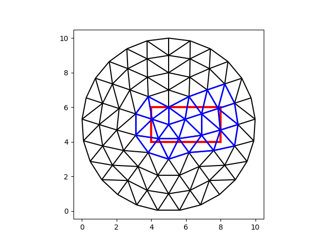
Locating bounding boxes

A search of N points will yield N answers (cell numbers). A search of N boxes may yield M answers. To illustrate, let’s look for all the cells inside of a box.

box_coords = np.array(
    [
        [4.0, 8.0, 4.0, 6.0],  # xmin, xmax, ymin, ymax
    ]
)
box_i, cell_i = tree.locate_boxes(box_coords)

fig, ax = plt.subplots()
demo.plot_edges(node_x, node_y, edges, ax, color="black")
demo.plot_edges(
    node_x, node_y, demo.edges(faces[cell_i], -1), ax, color="blue", linewidth=2
)
demo.plot_boxes(box_coords, ax, color="red", linewidth=3)

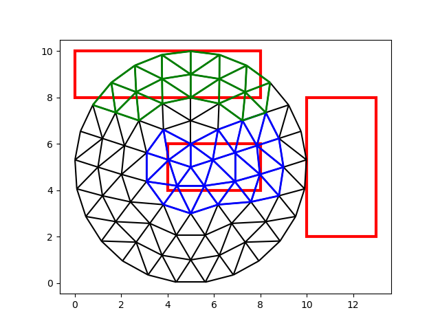
We can also search for multiple boxes:

box_coords = np.array(
    [
        [4.0, 8.0, 4.0, 6.0],
        [0.0, 8.0, 8.0, 10.0],
        [10.0, 13.0, 2.0, 8.0],
    ]
)
box_i, cell_i = tree.locate_boxes(box_coords)
box_i, cell_i

(array([0, 0, 0, 0, 0, 0, 0, 0, 0, 0, 0, 0, 0, 0, 0, 0, 0, 0, 0, 0, 0, 0,
       0, 0, 0, 0, 0, 0, 0, 0, 1, 1, 1, 1, 1, 1, 1, 1, 1, 1, 1, 1, 1, 1,
       1, 1, 1, 1, 1, 1, 1, 1, 1]), array([ 36,  37,  33,  34,  35,  84,  32,  89,  87,  90,  39,  20,  97,
        99,  98, 101, 102,  88,  44, 100,  31,  92,  91,  56,  55,  57,
        58,  63,  62,  64,  74,  23,  24,  76,  75,  25,  26,  29,  30,
        79,  80,  27,  28,  81,  82,  70,  69,  16,  17,  68,  14,  15,
        65]))

Note that this method returns two arrays of equal length. The second array contains the cell numbers, as usual. The first array contains the index of the bounding box in which the respective cells fall. Note that there are only two numbers in box_i: there are no cells located in the third box, as we can confirm visually:

cells_0 = cell_i[box_i == 0]
cells_1 = cell_i[box_i == 1]

fig, ax = plt.subplots()
demo.plot_edges(node_x, node_y, edges, ax, color="black")
demo.plot_edges(
    node_x, node_y, demo.edges(faces[cells_0], -1), ax, color="blue", linewidth=2
)
demo.plot_edges(
    node_x, node_y, demo.edges(faces[cells_1], -1), ax, color="green", linewidth=2
)
demo.plot_boxes(box_coords, ax, color="red", linewidth=3)

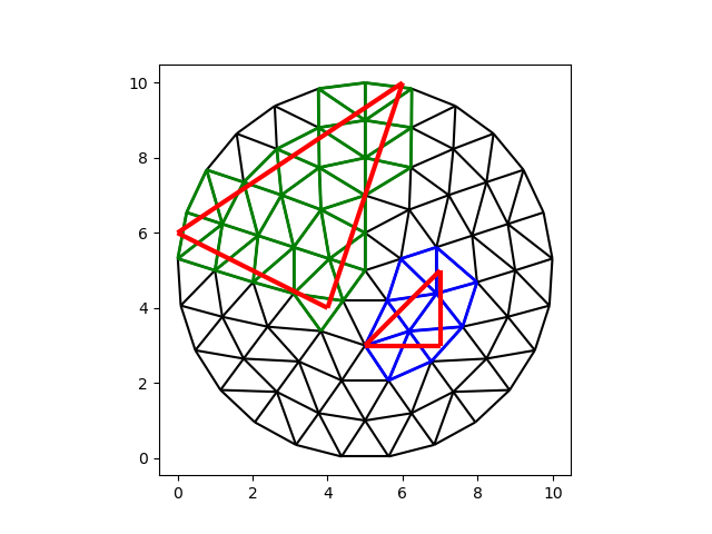
Locating cells

Similarly, we can look for other cells (convex polygons) and compute the overlap:

This returns three arrays of equal length:

• the index of the face to locate

• the index of the face in the celtree

• the area of the intersection

triangle_vertices = np.array(
    [
        [5.0, 3.0],
        [7.0, 3.0],
        [7.0, 5.0],
        [0.0, 6.0],
        [4.0, 4.0],
        [6.0, 10.0],
    ]
)
triangles = np.array(
    [
        [0, 1, 2],
        [3, 4, 5],
    ]
)
tri_x, tri_y = triangle_vertices.transpose()

tri_i, cell_i, area = tree.intersect_faces(triangle_vertices, triangles, -1)
cells_0 = cell_i[tri_i == 0]
cells_1 = cell_i[tri_i == 1]

fig, ax = plt.subplots()
demo.plot_edges(node_x, node_y, edges, ax, color="black")
demo.plot_edges(
    node_x, node_y, demo.edges(faces[cells_0], -1), ax, color="blue", linewidth=2
)
demo.plot_edges(
    node_x, node_y, demo.edges(faces[cells_1], -1), ax, color="green", linewidth=2
)
demo.plot_edges(tri_x, tri_y, demo.edges(triangles, -1), ax, color="red", linewidth=3)

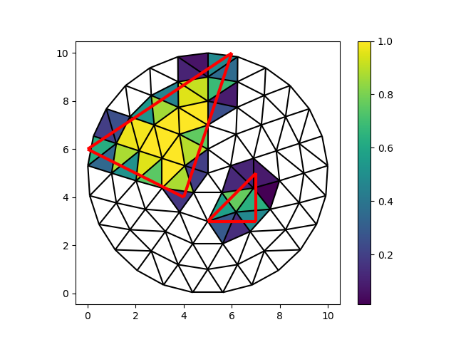
Let’s color the faces of the mesh by their ratio of overlap. Because our mesh is triangular, we can represent the triangles as two collections of vectors (V, U). Then the area is half of the absolute value of the cross product of U and V.

intersection_faces = faces[cell_i]
intersection_vertices = vertices[intersection_faces]
U = intersection_vertices[:, 1] - intersection_vertices[:, 0]
V = intersection_vertices[:, 2] - intersection_vertices[:, 0]
full_area = 0.5 * np.abs(np.cross(V, U))
ratio = area / full_area

fig, ax = plt.subplots()
colored = ax.tripcolor(
    node_x,
    node_y,
    intersection_faces,
    ratio,
)
fig.colorbar(colored)
demo.plot_edges(node_x, node_y, edges, ax, color="black")
demo.plot_edges(tri_x, tri_y, demo.edges(triangles, -1), ax, color="red", linewidth=3)

CellTree2d also provides a method to compute overlaps between boxes and a mesh. This may come in handy to compute overlap with a raster, for example to rasterize a mesh.

dx = 1.0
xmin = 0.0
xmax = 10.0

dy = -1.0
ymin = 0.0
ymax = 10.0

y, x = np.meshgrid(
    np.arange(ymax, ymin + dy, dy),
    np.arange(xmin, xmax + dx, dx),
    indexing="ij",
)
ny = y.shape[0] - 1
nx = x.shape[1] - 1
coords = np.column_stack(
    [a.ravel() for a in [x[:-1, :-1], x[1:, 1:], y[1:, 1:], y[:-1, :-1]]]
)
raster_i, cell_i, raster_overlap = tree.intersect_boxes(coords)

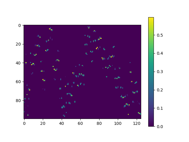
We can construct a weight matrix with these arrays. This weight matrix stores for every raster cell (row) the area of overlap with a triangle (column).

weight_matrix = np.zeros((ny * nx, len(faces)))
weight_matrix[raster_i, cell_i] = raster_overlap

fig, ax = plt.subplots()
colored = ax.imshow(weight_matrix)
_ = fig.colorbar(colored)

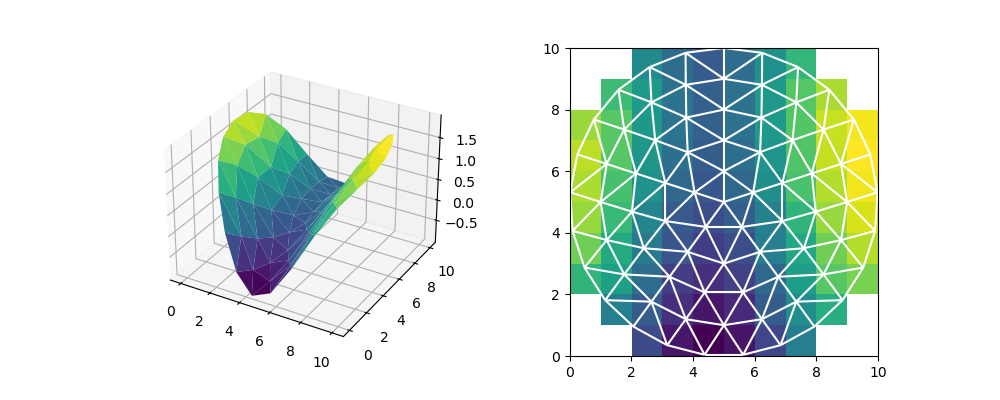
This weight matrix can be used for translating data from one mesh to another. Let’s generate some mock elevation data for a valley. Then, we’ll compute the area weighted mean for every raster cell.

def saddle_elevation(x, y):
    return np.sin(0.6 * x + 2) + np.sin(0.2 * y)


# Generate an elevation for every triangle
centroid_x, centroid_y = vertices[faces].mean(axis=1).transpose()
face_z = saddle_elevation(centroid_x, centroid_y)

# Compute the weighted mean of the triangles per raster cell
weighted_elevation = np.dot(weight_matrix, face_z)
area_sum = np.dot(weight_matrix, np.ones(len(faces)))
mean_elevation = np.full(ny * nx, np.nan)
intersects = area_sum > 0
mean_elevation[intersects] = weighted_elevation[intersects] / area_sum[intersects]

fig = plt.figure(figsize=(10, 4))
ax0 = fig.add_subplot(1, 2, 1, projection="3d")
ax0.plot_trisurf(
    node_x, node_y, faces, saddle_elevation(node_x, node_y), cmap="viridis"
)
ax1 = fig.add_subplot(1, 2, 2)
ax1.imshow(mean_elevation.reshape(ny, nx), extent=(xmin, xmax, ymin, ymax))
demo.plot_edges(node_x, node_y, edges, ax1, color="white")

Such a weight matrix doesn’t apply to just boxes and triangles, but to every case of mapping one mesh to another by intersecting cell areas. Note however that the aggregation above is not very efficient. Most of the entries in the weight matrix are 0; a raster cell only intersects a small number triangles. Such a matrix is much more efficiently stored and processed as a sparse matrix (see also Scipy sparse). The arrays returned by the intersect_ methods of CellTree2d form a coordinate list (COO).

Such a coordinate list can also be easily used to aggregate values with Pandas, as Pandas provides very efficient aggregation in the form of groupby operations.

Locating lines

As a final example, we will compute the intersections with two lines (edges). This once again returns three arrays of equal length:

• the index of the line

• the index of the cell

• the location of the intersection

edge_coords = np.array(
    [
        [[0.0, 0.0], [10.0, 10.0]],
        [[0.0, 10.0], [10.0, 0.0]],
    ]
)
edge_i, cell_i, intersections = tree.intersect_edges(edge_coords)
edge_i, cell_i

(array([0, 0, 0, 0, 0, 0, 0, 0, 0, 0, 0, 0, 0, 0, 0, 0, 0, 0, 1, 1, 1, 1,
       1, 1, 1, 1, 1, 1, 1, 1, 1, 1, 1, 1, 1, 1]), array([ 71,  23,  24,  25,  84,  86,  89,  87,  90,  55,  63,  64,  47,
        60, 118, 116, 117,  54, 105,  41,  40, 106, 103,  98, 101,  88,
       100,  16,  31,  92,  94,  96,  91,  14,  15,  65]))

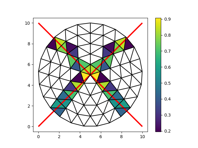
To wrap up, we’ll color the intersect faces with the length of the intersected line segments. We can easily compute the length of each segment with the Euclidian norm (Pythagorean distance):

length = np.linalg.norm(intersections[:, 1] - intersections[:, 0], axis=1)

fig, ax = plt.subplots()
colored = ax.tripcolor(
    node_x,
    node_y,
    faces[cell_i],
    length,
)
fig.colorbar(colored)
ax.add_collection(LineCollection(edge_coords, color="red", linewidth=3))
demo.plot_edges(node_x, node_y, edges, ax, color="black")