Tip

For an interactive online version click here:

Prepare flow directions and related data from a DEM

With HydroMT-Wflow, a user can choose to build a model in a geographic or projected coordinate system from an input Digital Elevation Model (DEM) and Flow Direction (flwdir) dataset.

While DEM data are often available, this is not the always the case for the flow directions (flwdir). We made the choice to build a Wflow model directly from user provided DEM and flwdir datasets rather than reprojecting a DEM and/or deriving flwdir on the fly. This is because deriving flow directions is often an iterative process to be sure the flow directions matche the terrain and river network. Note that for the best results the flwdir data should be derived from a high-res DEM (<100 m spatial resolution). The HydroMT-Wflow model builder will automatically resample the flwdir data to the model resolution.

Because of this, we prefer to provide this notebook as a possible pre-processing step before calling a build a Wflow model with HydroMt-Wflow. Here we use the different flow directions methods from HydroMT and PyFlwDir

Load dependencies

import os
import xarray as xr
import numpy as np
import geopandas as gpd

# pyflwdir
import pyflwdir

# hydromt
from hydromt import DataCatalog, flw

# plot
import matplotlib.pyplot as plt
from matplotlib import cm, colors
import cartopy.crs as ccrs

# we assume the model maps are in the geographic CRS EPSG:4326
proj = ccrs.PlateCarree()

# create nice elevation colormap
c_dem = plt.cm.terrain(np.linspace(0.25, 1, 256))
cmap = colors.LinearSegmentedColormap.from_list("dem", c_dem)
norm = colors.Normalize(vmin=0, vmax=2000)
kwargs = dict(cmap=cmap, norm=norm)

# legend settings
legend_kwargs = dict(
    title="Legend",
    loc="lower right",
    frameon=True,
    framealpha=0.7,
    edgecolor="k",
    facecolor="white",
)


def add_legend_titles(ax, title, add_legend=True, projected=True):
    ax.xaxis.set_visible(True)
    ax.yaxis.set_visible(True)
    if projected:
        ax.set_xlabel("Easting [m]")
        ax.set_ylabel("Northing [m]")
    else:
        ax.set_ylabel("latitude [degree north]")
        ax.set_xlabel("longitude [degree east]")
    _ = ax.set_title(title)
    if add_legend:
        legend = ax.legend(**legend_kwargs)

        return legend

Deriving flow directions from Elevation data

In this example we will use the merit_hydro data in the pre-defined artifact_data catalog of HydroMT. Note that this dataset already provides flow direction, but for sake of example we only use this as reference dataset.

First let’s read the data:

data_catalog = DataCatalog("artifact_data")
merit = data_catalog.get_rasterdataset(
    "merit_hydro", variables=["elevtn", "flwdir"], bbox=[12, 46.0, 12.3, 46.2]
)

Dataset does [12.000000000000016, 45.99999999999999, 12.300000000000011, 46.199999999999996] does not fully cover bbox [12.000, 46.000, 12.300, 46.200]

To derive flow directions from a DEM, you can use the hydromt.flw.d8_from_dem method of HydroMT.

This method derives D8 flow directions grid from an elevation grid and allows several options to the users: - outlets: outlets can be defined at edges of the grid (defualt) or force all flow to go to the minimum elevation point min. The latter only makes sense if your DEM only is masked to the catchment. Additionnally, the user can also force specific pits locations via idxs_pit. - depression filling: local depressions are filled based on their lowest pour point level if the pour point depth is smaller than the maximum pour point depth max_depth, otherwise the lowest elevation in the depression becomes a pit. By default max_depth is set to -1 m filling all local depressions. - river burning: while it is already possible to provide a river vector layer gdf_stream with uparea (km2) column to further guide the derivation of flow directions, this option is currently being improved and not yet fully functional. See also HydroMT core PR 305

Let’s see an example:

# Derive flow directions with outlets at the edges -> this is the default
merit["flwdir_derived"] = flw.d8_from_dem(
    da_elv=merit["elevtn"],
    gdf_stream=None,
    max_depth=-1,  # no local pits
    outlets="edge",
    idxs_pit=None,
)

# Get the CRS and check if it is projected or not
is_geographic = merit.raster.crs.is_geographic

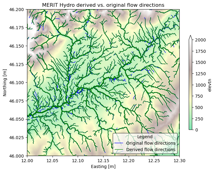
Let’s compare the orignal with the derived flow direction data

# plot
# initialize image with geoaxes
fig = plt.figure(figsize=(8, 8))
ax = fig.add_subplot()

## plot elevation\
merit["elevtn"].plot(
    ax=ax, zorder=1, cbar_kwargs=dict(aspect=30, shrink=0.5), alpha=0.5, **kwargs
)

# plot flwdir
flwdir = flw.flwdir_from_da(merit["flwdir"], ftype="infer", check_ftype=True)
feat = flwdir.streams(min_sto=3)  # minimum stream order for plotting
gdf = gpd.GeoDataFrame.from_features(feat, crs=merit.raster.crs)
gdf.to_crs(merit.raster.crs).plot(
    ax=ax, color="blue", linewidth=gdf["strord"] / 3, label="Original flow directions"
)


# plot flwdir edge
flwdir_edge = flw.flwdir_from_da(
    merit["flwdir_derived"], ftype="infer", check_ftype=True
)
feate = flwdir_edge.streams(min_sto=3)  # minimum stream order for plotting
gdfe = gpd.GeoDataFrame.from_features(feate, crs=merit.raster.crs)
gdfe.plot(
    ax=ax,
    column="strord",
    color="green",
    linewidth=gdfe["strord"] / 3,
    label="Derived flow directions",
)

legend = add_legend_titles(ax, "MERIT Hydro derived vs. original flow directions")

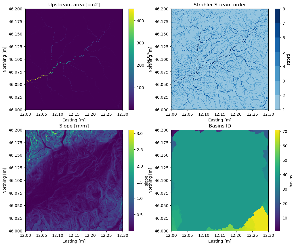
Deriving other DEM and flow directions related data

Once you are satisfied with your flow direction map, you can create additionnal derived variables like upstream area or streamorder that can prove useful for example to build a model based on subbasin region.

Here are some examples how to do that using PyFlwdir methods.

# Create a new merit_adapted dataset with the riverburn flow directions
merit_adapted = merit["elevtn"].to_dataset(name="elevtn")
merit_adapted["flwdir"] = merit["flwdir_derived"]
dims = merit_adapted.raster.dims

# Create a PyFlwDir object from the dataset
flwdir = flw.flwdir_from_da(merit_adapted["flwdir"])

# uparea
uparea = flwdir.upstream_area(unit="km2")
merit_adapted["uparea"] = xr.Variable(dims, uparea, attrs=dict(_FillValue=-9999))

# stream order
strord = flwdir.stream_order()
merit_adapted["strord"] = xr.Variable(dims, strord)
merit_adapted["strord"].raster.set_nodata(255)

# slope
slope = pyflwdir.dem.slope(
    elevtn=merit_adapted["elevtn"].values,
    nodata=merit_adapted["elevtn"].raster.nodata,
    latlon=is_geographic,  # True if geographic crs, False if projected crs
    transform=merit_adapted["elevtn"].raster.transform,
)
merit_adapted["slope"] = xr.Variable(dims, slope)
merit_adapted["slope"].raster.set_nodata(merit_adapted["elevtn"].raster.nodata)

# basin at the pits locations
basins = flwdir.basins(idxs=flwdir.idxs_pit).astype(np.int32)
merit_adapted["basins"] = xr.Variable(dims, basins, attrs=dict(_FillValue=0))

# basin index file
gdf_basins = merit_adapted["basins"].raster.vectorize()

merit_adapted

<xarray.Dataset>
Dimensions:      (x: 360, y: 240)
Coordinates:
  * x            (x) float64 12.0 12.0 12.0 12.0 12.0 ... 12.3 12.3 12.3 12.3
  * y            (y) float64 46.2 46.2 46.2 46.2 46.2 ... 46.0 46.0 46.0 46.0
    spatial_ref  int64 0
Data variables:
    elevtn       (y, x) float32 dask.array<chunksize=(240, 360), meta=np.ndarray>
    flwdir       (y, x) uint8 0 16 1 0 16 1 1 0 16 ... 0 16 16 16 16 1 0 16 16
    uparea       (y, x) float64 0.2199 0.005943 0.005943 ... 0.2326 0.005965
    strord       (y, x) uint8 2 1 1 2 1 1 2 3 2 1 1 2 ... 6 1 3 3 3 2 1 1 3 2 1
    slope        (y, x) float32 0.5143 0.5413 0.2722 ... 0.1841 0.1583 0.1146
    basins       (y, x) int32 1 1 2 2 2 3 3 3 3 3 ... 70 70 70 70 70 71 71 71 71

xarray.Dataset

• Dimensions:
  • x: 360
  • y: 240
• Coordinates: (3)
  • x
    (x)
    float64
    12.0 12.0 12.0 ... 12.3 12.3 12.3

    array([12.000417, 12.00125 , 12.002083, ..., 12.297917, 12.29875 , 12.299583])

  • y
    (y)
    float64
    46.2 46.2 46.2 ... 46.0 46.0 46.0

    array([46.199583, 46.19875 , 46.197917, ..., 46.002083, 46.00125 , 46.000417])

  • spatial_ref
    ()
    int64
    0

    crs_wkt :

    GEOGCRS["WGS 84",DATUM["World Geodetic System 1984",ELLIPSOID["WGS 84",6378137,298.257223563,LENGTHUNIT["metre",1]]],PRIMEM["Greenwich",0,ANGLEUNIT["degree",0.0174532925199433]],CS[ellipsoidal,2],AXIS["geodetic latitude (Lat)",north,ORDER[1],ANGLEUNIT["degree",0.0174532925199433]],AXIS["geodetic longitude (Lon)",east,ORDER[2],ANGLEUNIT["degree",0.0174532925199433]],ID["EPSG",4326]]

    semi_major_axis :

    6378137.0

    semi_minor_axis :

    6356752.314245179

    inverse_flattening :

    298.257223563

    reference_ellipsoid_name :

    WGS 84

    longitude_of_prime_meridian :

    0.0

    prime_meridian_name :

    Greenwich

    geographic_crs_name :

    WGS 84

    horizontal_datum_name :

    World Geodetic System 1984

    grid_mapping_name :

    latitude_longitude

    spatial_ref :

    GEOGCRS["WGS 84",DATUM["World Geodetic System 1984",ELLIPSOID["WGS 84",6378137,298.257223563,LENGTHUNIT["metre",1]]],PRIMEM["Greenwich",0,ANGLEUNIT["degree",0.0174532925199433]],CS[ellipsoidal,2],AXIS["geodetic latitude (Lat)",north,ORDER[1],ANGLEUNIT["degree",0.0174532925199433]],AXIS["geodetic longitude (Lon)",east,ORDER[2],ANGLEUNIT["degree",0.0174532925199433]],ID["EPSG",4326]]

    GeoTransform :

    11.600000000000023 0.0008333333333333203 0.0 46.8 0.0 -0.0008333333333333345

    x_dim :

    x

    y_dim :

    y

    array(0)

• Data variables: (6)
  • elevtn
    (y, x)
    float32
    dask.array<chunksize=(240, 360), meta=np.ndarray>

    AREA_OR_POINT :

    Area

    _FillValue :

    -9999.0

    source_file :

    elevtn.tif

    Array Chunk Bytes 337.50 kiB 337.50 kiB Shape (240, 360) (240, 360) Dask graph 1 chunks in 4 graph layers Data type float32 numpy.ndarray

  • flwdir
    (y, x)
    uint8
    0 16 1 0 16 1 1 ... 16 16 1 0 16 16

    _FillValue :

    247

    array([[  0,  16,   1, ...,   2,   2,   4],
           [ 64,  32, 128, ...,   2,   2,   4],
           [ 64,  32,  32, ...,   4,   8,   8],
           ...,
           [ 64,  32, 128, ...,   8,   2,   4],
           [ 64,  32,  32, ...,   4,   8,   8],
           [ 64,  32,  32, ...,   0,  16,  16]], dtype=uint8)

  • uparea
    (y, x)
    float64
    0.2199 0.005943 ... 0.2326 0.005965

    _FillValue :

    -9999

    array([[0.21991321, 0.00594301, 0.00594301, ..., 0.00594301, 0.00594301,
            0.00594301],
           [0.19614088, 0.0118863 , 0.0059431 , ..., 0.0059431 , 0.01188612,
            0.01782913],
           [0.1783113 , 0.01188648, 0.00594319, ..., 0.00594319, 0.0118863 ,
            0.03565844],
           ...,
           [0.03578676, 0.01789329, 0.00596434, ..., 0.00596434, 0.00596434,
            0.20873662],
           [0.01789347, 0.01192895, 0.01192895, ..., 0.00596443, 0.00596443,
            0.22066539],
           [0.00596452, 0.00596452, 0.00596452, ..., 0.34591481, 0.23259443,
            0.00596452]])

  • strord
    (y, x)
    uint8
    2 1 1 2 1 1 2 3 ... 3 3 2 1 1 3 2 1

    _FillValue :

    255

    array([[2, 1, 1, ..., 1, 1, 1],
           [2, 1, 1, ..., 1, 1, 2],
           [2, 1, 1, ..., 1, 1, 2],
           ...,
           [2, 1, 1, ..., 1, 1, 2],
           [2, 1, 1, ..., 1, 1, 2],
           [1, 1, 1, ..., 3, 2, 1]], dtype=uint8)

  • slope
    (y, x)
    float32
    0.5143 0.5413 ... 0.1583 0.1146

    _FillValue :

    -9999.0

    array([[0.51432776, 0.5413488 , 0.27221325, ..., 0.00747009, 0.02149446,
            0.01136101],
           [0.5459833 , 0.80539113, 0.6450317 , ..., 0.02068615, 0.03458828,
            0.02887675],
           [0.474031  , 0.8115524 , 0.6958318 , ..., 0.05807183, 0.01134925,
            0.02159704],
           ...,
           [0.17576262, 0.2855775 , 0.30759504, ..., 0.12126302, 0.11745112,
            0.11047088],
           [0.22475238, 0.34088627, 0.27726272, ..., 0.17765708, 0.21685791,
            0.15327132],
           [0.10499322, 0.23972316, 0.17005979, ..., 0.18411785, 0.1582703 ,
            0.1145691 ]], dtype=float32)

  • basins
    (y, x)
    int32
    1 1 2 2 2 3 3 ... 70 70 71 71 71 71

    _FillValue :

    0

    array([[ 1,  1,  2, ..., 21, 21, 21],
           [ 1,  1,  2, ..., 21, 21, 21],
           [ 1,  1,  1, ..., 21, 21, 21],
           ...,
           [48, 48, 48, ..., 71, 71, 71],
           [48, 48, 48, ..., 71, 71, 71],
           [48, 48, 48, ..., 71, 71, 71]], dtype=int32)

• Indexes: (2)
  • x
    PandasIndex

    PandasIndex(Index([12.000416666666682, 12.001250000000017,  12.00208333333335,
           12.002916666666682, 12.003750000000016, 12.004583333333349,
           12.005416666666683, 12.006250000000016, 12.007083333333348,
           12.007916666666683,
           ...
           12.292083333333345, 12.292916666666677, 12.293750000000012,
           12.294583333333344, 12.295416666666679, 12.296250000000011,
           12.297083333333344, 12.297916666666678,  12.29875000000001,
           12.299583333333345],
          dtype='float64', name='x', length=360))

  • y
    PandasIndex

    PandasIndex(Index([ 46.19958333333333,           46.19875, 46.197916666666664,
            46.19708333333333,           46.19625,  46.19541666666667,
            46.19458333333333, 46.193749999999994,  46.19291666666666,
            46.19208333333333,
           ...
            46.00791666666667,  46.00708333333333, 46.006249999999994,
            46.00541666666666,  46.00458333333333,           46.00375,
           46.002916666666664,  46.00208333333333,           46.00125,
           46.000416666666666],
          dtype='float64', name='y', length=240))

• Attributes: (0)

# plot
fig, axes = plt.subplots(2, 2, figsize=(12, 10))

# plot uparea
merit_adapted["uparea"].plot(ax=axes[0, 0])
_ = add_legend_titles(axes[0, 0], "Upstream area [km2]", add_legend=False)

# plot strord
merit_adapted["strord"].plot(
    ax=axes[0, 1], cmap=colors.ListedColormap(cm.Blues(np.linspace(0.4, 1, 7)))
)
_ = add_legend_titles(axes[0, 1], "Strahler Stream order", add_legend=False)

# plot slope
merit_adapted["slope"].plot(ax=axes[1, 0])
_ = add_legend_titles(axes[1, 0], "Slope [m/m]", add_legend=False)

# plot basins
merit_adapted["basins"].plot(ax=axes[1, 1])
_ = add_legend_titles(axes[1, 1], "Basins ID", add_legend=False)

Exporting the newly created data and corresponding data catalog

Finally, once we are happy with the new dataset, we can write out the data and create the corresponding data catalog so that it can be re-used to build a new wflow model.

# Export the gridded data as tif files in a new folder
output_path = "./elevation_data"

# export the hydrography data as tif files (one per variable)
merit_adapted.raster.to_mapstack(
    root=os.path.join(output_path, "merit_adapted"),
    driver="GTiff",
)

# export the basin index as geosjon
gdf_basins.to_file(
    os.path.join(output_path, "merit_adapted_basins.geojson"), driver="GeoJSON"
)

Now let’s prepare the corresponding data catalog: (the writefile command will directly write a file using the lines in the jupyter cell)

%%writefile ./elevation_data/data_catalog.yml
merit_adapted:
  data_type: RasterDataset
  driver: raster
  crs: 3857
  path: ./merit_adapted/{variable}.tif
  rename:
    slope: lndslp
  meta:
    category: topography
    paper_doi: 10.5194/hess-2020-582
    paper_ref: Eilander et al. (2021)
    source_license: ODC-By 1.0
    source_url: https://zenodo.org/record/5166932#.YVbxJ5pByUk
    source_doi: 10.5281/zenodo.5166932
    source_version: 1.0
    processing_notes: prepared from MERIT Hydro IHU by deriving flow directions with river burning from lin2019_v1 rivers using pyflwdir.
    processing_script: prepare_ldd.ipynb from hydromt_wflow repository

merit_adapted_index:
  data_type: GeoDataFrame
  driver: vector
  crs: 3857
  path: ./merit_adapted_basins.geojson
  meta:
    category: topography
    paper_doi: 10.5194/hess-2020-582
    paper_ref: Eilander et al. (2021)
    source_license: ODC-By 1.0
    source_url: https://zenodo.org/record/5166932#.YVbxJ5pByUk
    source_doi: 10.5281/zenodo.5166932
    source_version: 1.0
    processing_notes: prepared from MERIT Hydro IHU by deriving flow directions with river burning from lin2019_v1 rivers using pyflwdir.
    processing_script: prepare_ldd.ipynb from hydromt_wflow repository

Writing ./elevation_data/data_catalog.yml

And now let’s try to load our data again with hydromt:

data_catalog = DataCatalog(data_libs="./elevation_data/data_catalog.yml")

merit_utm = data_catalog.get_rasterdataset("merit_adapted")
merit_utm

RasterDataset merit_adapted: CRS from data catalog does not match CRS  of data. The original CRS will be used. Please check your catalog.

<xarray.Dataset>
Dimensions:      (x: 360, y: 240)
Coordinates:
  * x            (x) float64 12.0 12.0 12.0 12.0 12.0 ... 12.3 12.3 12.3 12.3
  * y            (y) float64 46.2 46.2 46.2 46.2 46.2 ... 46.0 46.0 46.0 46.0
    spatial_ref  int64 0
Data variables:
    basins       (y, x) int32 dask.array<chunksize=(240, 360), meta=np.ndarray>
    elevtn       (y, x) float32 dask.array<chunksize=(240, 360), meta=np.ndarray>
    flwdir       (y, x) uint8 dask.array<chunksize=(240, 360), meta=np.ndarray>
    lndslp       (y, x) float32 dask.array<chunksize=(240, 360), meta=np.ndarray>
    strord       (y, x) uint8 dask.array<chunksize=(240, 360), meta=np.ndarray>
    uparea       (y, x) float64 dask.array<chunksize=(240, 360), meta=np.ndarray>
Attributes:
    category:           topography
    paper_doi:          10.5194/hess-2020-582
    paper_ref:          Eilander et al. (2021)
    source_license:     ODC-By 1.0
    source_url:         https://zenodo.org/record/5166932#.YVbxJ5pByUk
    source_doi:         10.5281/zenodo.5166932
    source_version:     1.0
    processing_notes:   prepared from MERIT Hydro IHU by deriving flow direct...
    processing_script:  prepare_ldd.ipynb from hydromt_wflow repository

xarray.Dataset

• Dimensions:
  • x: 360
  • y: 240
• Coordinates: (3)
  • x
    (x)
    float64
    12.0 12.0 12.0 ... 12.3 12.3 12.3

    array([12.000417, 12.00125 , 12.002083, ..., 12.297917, 12.29875 , 12.299583])

  • y
    (y)
    float64
    46.2 46.2 46.2 ... 46.0 46.0 46.0

    array([46.199583, 46.19875 , 46.197917, ..., 46.002083, 46.00125 , 46.000417])

  • spatial_ref
    ()
    int64
    0

    crs_wkt :

    GEOGCRS["WGS 84",DATUM["World Geodetic System 1984",ELLIPSOID["WGS 84",6378137,298.257223563,LENGTHUNIT["metre",1]]],PRIMEM["Greenwich",0,ANGLEUNIT["degree",0.0174532925199433]],CS[ellipsoidal,2],AXIS["geodetic latitude (Lat)",north,ORDER[1],ANGLEUNIT["degree",0.0174532925199433]],AXIS["geodetic longitude (Lon)",east,ORDER[2],ANGLEUNIT["degree",0.0174532925199433]],ID["EPSG",4326]]

    semi_major_axis :

    6378137.0

    semi_minor_axis :

    6356752.314245179

    inverse_flattening :

    298.257223563

    reference_ellipsoid_name :

    WGS 84

    longitude_of_prime_meridian :

    0.0

    prime_meridian_name :

    Greenwich

    geographic_crs_name :

    WGS 84

    horizontal_datum_name :

    World Geodetic System 1984

    grid_mapping_name :

    latitude_longitude

    spatial_ref :

    GEOGCRS["WGS 84",DATUM["World Geodetic System 1984",ELLIPSOID["WGS 84",6378137,298.257223563,LENGTHUNIT["metre",1]]],PRIMEM["Greenwich",0,ANGLEUNIT["degree",0.0174532925199433]],CS[ellipsoidal,2],AXIS["geodetic latitude (Lat)",north,ORDER[1],ANGLEUNIT["degree",0.0174532925199433]],AXIS["geodetic longitude (Lon)",east,ORDER[2],ANGLEUNIT["degree",0.0174532925199433]],ID["EPSG",4326]]

    GeoTransform :

    12.000000000000016 0.0008333333333333225 0.0 46.199999999999996 0.0 -0.0008333333333333186

    x_dim :

    x

    y_dim :

    y

    array(0)

• Data variables: (6)
  • basins
    (y, x)
    int32
    dask.array<chunksize=(240, 360), meta=np.ndarray>

    AREA_OR_POINT :

    Area

    _FillValue :

    0

    source_file :

    basins.tif

    Array Chunk Bytes 337.50 kiB 337.50 kiB Shape (240, 360) (240, 360) Dask graph 1 chunks in 3 graph layers Data type int32 numpy.ndarray

  • elevtn
    (y, x)
    float32
    dask.array<chunksize=(240, 360), meta=np.ndarray>

    AREA_OR_POINT :

    Area

    _FillValue :

    -9999.0

    source_file :

    elevtn.tif

    Array Chunk Bytes 337.50 kiB 337.50 kiB Shape (240, 360) (240, 360) Dask graph 1 chunks in 3 graph layers Data type float32 numpy.ndarray

  • flwdir
    (y, x)
    uint8
    dask.array<chunksize=(240, 360), meta=np.ndarray>

    AREA_OR_POINT :

    Area

    _FillValue :

    247

    source_file :

    flwdir.tif

    Array Chunk Bytes 84.38 kiB 84.38 kiB Shape (240, 360) (240, 360) Dask graph 1 chunks in 3 graph layers Data type uint8 numpy.ndarray

  • lndslp
    (y, x)
    float32
    dask.array<chunksize=(240, 360), meta=np.ndarray>

    AREA_OR_POINT :

    Area

    _FillValue :

    -9999.0

    source_file :

    slope.tif

    Array Chunk Bytes 337.50 kiB 337.50 kiB Shape (240, 360) (240, 360) Dask graph 1 chunks in 3 graph layers Data type float32 numpy.ndarray

  • strord
    (y, x)
    uint8
    dask.array<chunksize=(240, 360), meta=np.ndarray>

    AREA_OR_POINT :

    Area

    _FillValue :

    255

    source_file :

    strord.tif

    Array Chunk Bytes 84.38 kiB 84.38 kiB Shape (240, 360) (240, 360) Dask graph 1 chunks in 3 graph layers Data type uint8 numpy.ndarray

  • uparea
    (y, x)
    float64
    dask.array<chunksize=(240, 360), meta=np.ndarray>

    AREA_OR_POINT :

    Area

    _FillValue :

    -9999.0

    source_file :

    uparea.tif

    Array Chunk Bytes 675.00 kiB 675.00 kiB Shape (240, 360) (240, 360) Dask graph 1 chunks in 3 graph layers Data type float64 numpy.ndarray

• Indexes: (2)
  • x
    PandasIndex

    PandasIndex(Index([12.000416666666682, 12.001250000000015,  12.00208333333335,
           12.002916666666682, 12.003750000000016, 12.004583333333349,
           12.005416666666683, 12.006250000000016, 12.007083333333348,
           12.007916666666683,
           ...
           12.292083333333345,  12.29291666666668, 12.293750000000012,
           12.294583333333344, 12.295416666666679, 12.296250000000011,
           12.297083333333346, 12.297916666666678, 12.298750000000013,
           12.299583333333345],
          dtype='float64', name='x', length=360))

  • y
    PandasIndex

    PandasIndex(Index([ 46.19958333333333,           46.19875, 46.197916666666664,
            46.19708333333333,           46.19625,  46.19541666666666,
            46.19458333333333, 46.193749999999994,  46.19291666666666,
            46.19208333333333,
           ...
            46.00791666666667, 46.007083333333334,           46.00625,
            46.00541666666667, 46.004583333333336,           46.00375,
           46.002916666666664,  46.00208333333333,           46.00125,
           46.000416666666666],
          dtype='float64', name='y', length=240))

• Attributes: (9)

  category :

  topography

  paper_doi :

  10.5194/hess-2020-582

  paper_ref :

  Eilander et al. (2021)

  source_license :

  ODC-By 1.0

  source_url :

  https://zenodo.org/record/5166932#.YVbxJ5pByUk

  source_doi :

  10.5281/zenodo.5166932

  source_version :

  1.0

  processing_notes :

  prepared from MERIT Hydro IHU by deriving flow directions with river burning from lin2019_v1 rivers using pyflwdir.

  processing_script :

  prepare_ldd.ipynb from hydromt_wflow repository