Tip
SFINCS results: determine maximum water depth#
This notebook contains 2 examples, one for a standard regular SFINCS model, and one for a subgrid SFINCS model.
IMPORTANT NOTE, the methods for producing a flood depth map for the regular vs subgrid versions of SFINCS are NOT the same, and NOT interchangeable!
Contents: 1. Determine maximum water depth for a regular model 2. Determine maximum water depth for a subgrid model
1. Determine maximum water depth for a regular model#
The first example used in this notebook is based on a regular SFINCS model, i.e. no subgrid tables are used. In the absence of the subgrid tables, SFINCS computes the water depth by simply substracting the bed levels from the water levels. The (maximum) water depth h(max) is stored in the NetCDF output (sfincs_map.nc).
How to derive maximum water depths for a model including subgrid tables is explained later in this notebook.
[1]:
from os.path import join
import matplotlib.pyplot as plt
from hydromt_sfincs import SfincsModel, utils
Read model results#
The model results in sfincs_map.nc are saved as in a staggered grid format, see SGRID convention. Here we show how to retrieve the face values and translate the dimensions from node indices (m, n) to (x, y) coordinates in order to plot the results on a map.
[2]:
sfincs_root = "sfincs_compound"  # (relative) path to sfincs root
mod = SfincsModel(sfincs_root, mode="r")
[3]:
# we can simply read the model results (sfincs_map.nc and sfincs_his.nc) using the read_results method
mod.read_results()
# the following variables have been found
list(mod.results.keys())
[3]:
['inp',
 'msk',
 'zb',
 'zs',
 'h',
 'zsmax',
 'hmax',
 'total_runtime',
 'average_dt',
 'point_zb',
 'point_zs',
 'point_h']
[4]:
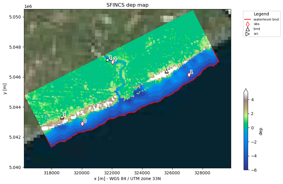
# plot the model layout
fig, ax = mod.plot_basemap(fn_out=None, bmap="sat", figsize=(11, 7))
Write maximum waterdepth to geotiff file#
[5]:
# uncomment to write hmax to <mod.root>/gis/hmax.tif
# mod.write_raster("results.hmax", compress="LZW")
Plot maximum water depth with surface water mask#
First we mask the water depth based on a map of permanent water to get the flood extent. The mask is calculated from the Global Surface Water Occurence (GSWO) dataset.
[6]:
# read global surface water occurance (GSWO) data to mask permanent water
mod.data_catalog.from_artifacts()
print(mod.data_catalog["gswo"])
gswo = mod.data_catalog.get_rasterdataset("gswo", geom=mod.region, buffer=10)

# NOTE to read data for a different region than Northen Italy add this data to the data catalog:
# mod.data_catalog.from_yml('/path/to/data_catalog.yml')

# permanent water where water occurence > 5%
gswo_mask = gswo.raster.reproject_like(mod.grid, method="max") <= 5
---------------------------------------------------------------------------
AttributeError                            Traceback (most recent call last)
Cell In[6], line 2
      1 # read global surface water occurance (GSWO) data to mask permanent water
----> 2 mod.data_catalog.from_artifacts()
      3 print(mod.data_catalog["gswo"])
      4 gswo = mod.data_catalog.get_rasterdataset("gswo", geom=mod.region, buffer=10)

AttributeError: 'DataCatalog' object has no attribute 'from_artifacts'
[7]:
hmin = 0.05  # minimum flood depth [m] to plot

# hmax is computed by SFINCS and read-in from the sfincs_map.nc file
da_hmax = mod.results["hmax"]

# get overland flood depth with GSWO and set minimum flood depth
da_hmax = da_hmax.where(gswo_mask).where(da_hmax > hmin)

# update attributes for colorbar label later
da_hmax.attrs.update(long_name="flood depth", unit="m")
---------------------------------------------------------------------------
NameError                                 Traceback (most recent call last)
Cell In[7], line 7
      4 da_hmax = mod.results["hmax"]
      6 # get overland flood depth with GSWO and set minimum flood depth
----> 7 da_hmax = da_hmax.where(gswo_mask).where(da_hmax > hmin)
      9 # update attributes for colorbar label later
     10 da_hmax.attrs.update(long_name="flood depth", unit="m")

NameError: name 'gswo_mask' is not defined
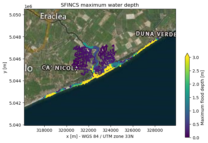
Here we plot the maximum water depth on top of the plot_basemap method to also include the locations of discharge source points and observation gauge locations.
[8]:
# create hmax plot and save to mod.root/figs/hmax.png
fig, ax = mod.plot_basemap(
    fn_out=None,
    figsize=(8, 6),
    variable=da_hmax,
    plot_bounds=False,
    plot_geoms=False,
    bmap="sat",
    zoomlevel=12,
    vmin=0,
    vmax=3.0,
    cmap=plt.cm.viridis,
    cbar_kwargs={"shrink": 0.6, "anchor": (0, 0)},
)
ax.set_title(f"SFINCS maximum water depth")
# plt.savefig(join(mod.root, 'figs', 'hmax.png'), dpi=225, bbox_inches="tight")
[8]:
Text(0.5, 1.0, 'SFINCS maximum water depth')
2. Determine maximum water depth for a subgrid model#
When subgrid tables are used, these are based on elevation data of a resolution higher than the resolution of the computational grid. The bed levels stored in the NetCDF output (zb in sfincs_map.nc) are the minimum bed levels from the subgrid tables of each computational cell. Therefore, to properly derive water depths, the higher resolution elevation data should be used instead of simply using the bed levels from the model output (this would result in an overestimation of flood extents). The process of interpolating the water levels onto the higher-resolution elevation data is called downscaling.
The downscaling of the floodmap roughly includees the following steps:
Select your high-resolution elevation dataset
Retrieve the maximum water levels from your model
Determine if and how you want to mask your floodmap
Write a geotiff of your downscaled floodmap
Plot your downscaled floodmap here, or in QGIS
[9]:
# select the example model
sfincs_root = "sfincs_compound"  # (relative) path to sfincs root
mod = SfincsModel(sfincs_root, mode="r")
In the example, we used GEBCO (~450m resolution) and MERIT Hydro (~90m resolution) to create a model on 50 meters resolution. In this case, including subgrid tables didn’t add much information to the model. To still illustrate the process of downscaling, we will use the dep.tif (in the gis folder) which has 50m resolution.
When creating a subgrid with setup_subgrid, you can easily create a geotiff on the subgrid resolution in the subgrid folder with the argument write_dep_tif=True.
[10]:
# first we are going to select our highest-resolution elevation dataset
depfile = join(sfincs_root, "gis", "dep.tif")

# with the depfile on subgrid resolution this would be:
# depfile = join(sfincs_root, "subgrid", "dep_subgrid.tif")

da_dep = mod.data_catalog.get_rasterdataset(depfile)
[11]:
# secondly we are reading in the model results
mod.read_results()

# now assuming we have a subgrid model, we don't have hmax available, so we are using zsmax (maximum water levels)
# compute the maximum over all time steps
da_zsmax = mod.results["zsmax"].max(dim="timemax")
[12]:
# thirdly, we determine the masking of the floodmap

# we could use the GSWO dataset to mask permanent water in a similar way as above
# NOTE: this is masking the water levels on the computational grid resolution

# alternatively we could use a geodataframe (e.g. OpenStreetMap landareas) to mask water bodies
# NOTE: small rivers are not masked with this geodataframe
gdf_osm = mod.data_catalog.get_geodataframe("osm_landareas")

# and again, we can use a threshold to mask minimum flood depth
hmin = 0.05
[13]:
# Fourthly, we downscale the floodmap
da_hmax = utils.downscale_floodmap(
    zsmax=da_zsmax,
    dep=da_dep,
    hmin=hmin,
    gdf_mask=gdf_osm,
    # floodmap_fn=join(sfincs_root, "floodmap.tif") # uncomment to save to <mod.root>/floodmap.tif
)
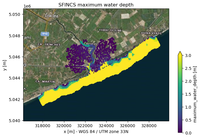
[14]:
# Lastly, we create a basemap plot with hmax on top
fig, ax = mod.plot_basemap(
    fn_out=None,
    figsize=(8, 6),
    variable=da_hmax,
    plot_bounds=False,
    plot_geoms=False,
    bmap="sat",
    zoomlevel=11,
    vmin=0,
    vmax=3.0,
    cbar_kwargs={"shrink": 0.6, "anchor": (0, 0)},
)
ax.set_title(f"SFINCS maximum water depth")
# plt.savefig(join(mod.root, 'figs', 'hmax.png'), dpi=225, bbox_inches="tight")
[14]:
Text(0.5, 1.0, 'SFINCS maximum water depth')