Tip

For an interactive online version click here:

Sfincs results: animation

The example used in this notebook is based on a regular SFINCS model, i.e. no subgrid tables are used. In the absence of the subgrid tables, SFINCS computes the water depth by simply substracting the bed levels from the water levels. The (maximum) water depth h(max) is stored in the NetCDF output (sfincs_map.nc).

How to derive maximum water depths for a model including subgrid tables is explained in a notebook about maximum water depths. A similar downscaling approach should be applied while making animations of a subgrid model!

# import dependencies
import numpy as np
import matplotlib.pyplot as plt
from hydromt_sfincs import SfincsModel

We use the cartopy package to plot maps. This packages provides a simple interface to plot geographic data and add background satellite imagery.

Read model results

The model results in sfincs_map.nc are saved as in a staggered grid format, see SGRID convention. Here we show how to retrieve the face values and translate the dimensions from node indices (m, n) to (x, y) coordinates in order to plot the results on a map.

sfincs_root = "sfincs_compound"  # (relative) path to sfincs root
mod = SfincsModel(sfincs_root, mode="r")

No region component found in components.

# we can simply read the model results (sfincs_map.nc and sfincs_his.nc) using the read_results method
mod.output.read()

/home/runner/work/hydromt_sfincs/hydromt_sfincs/hydromt_sfincs/components/grid/regulargrid.py:215: FutureWarning: In a future version of xarray the default value for compat will change from compat='no_conflicts' to compat='override'. This is likely to lead to different results when combining overlapping variables with the same name. To opt in to new defaults and get rid of these warnings now use `set_options(use_new_combine_kwarg_defaults=True) or set compat explicitly.
  ds = xr.merge(da_lst)
/home/runner/work/hydromt_sfincs/hydromt_sfincs/hydromt_sfincs/components/grid/regulargrid.py:215: FutureWarning: In a future version of xarray the default value for compat will change from compat='no_conflicts' to compat='override'. This is likely to lead to different results when combining overlapping variables with the same name. To opt in to new defaults and get rid of these warnings now use `set_options(use_new_combine_kwarg_defaults=True) or set compat explicitly.
  ds = xr.merge(da_lst)
Replacing result: inp
Replacing result: msk
Replacing result: zb
Replacing result: zs
Replacing result: h
Replacing result: zsmax
Replacing result: hmax
Replacing result: total_runtime
Replacing result: average_dt
Replacing result: status

Plot instantaneous water depths

# h from sfincs_map contains the water depths for each cell face
# here we plot the water level every 4th hour
h = mod.output.data["h"].where(mod.output.data["h"] > 0)
h.attrs.update(long_name="water depth", unit="m")
h.sel(time=h["time"].values[4::4]).plot(col="time", col_wrap=3, vmax=4)

<xarray.plot.facetgrid.FacetGrid at 0x7f84ab10f750>

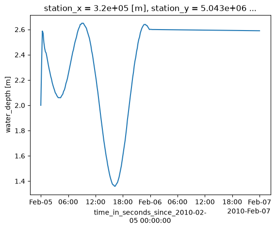
# point_h contains the water depths at the sfincs.obs gauge locations
# see mod.plot_basemaps (or next figure) for the location of the observation points
h_point = mod.output.data["point_h"].rename({"stations": "station_id"})
h_point["station_id"] = h_point["station_id"].astype(int)

# plot the water level at the first gauge
_ = h_point.sel({"station_id": 1}).plot.line(
    x="time",
)

/tmp/ipykernel_5527/3816678588.py:3: UserWarning: rename 'stations' to 'station_id' does not create an index anymore. Try using swap_dims instead or use set_index after rename to create an indexed coordinate.
  h_point = mod.output.data["point_h"].rename({"stations": "station_id"})

Create animation

An animation is also simple to make with matplotlib.animation method. Here we add the surface water level in blue colors next to the overland flood depth with viridis colormap.

# mask water depth
hmin = 0.05
da_h = mod.output.data["h"].copy()
da_h = da_h.where(da_h > hmin).drop("spatial_ref")
da_h.attrs.update(long_name="flood depth", unit="m")

/tmp/ipykernel_5527/2073427967.py:4: FutureWarning: dropping variables using `drop` is deprecated; use drop_vars.
  da_h = da_h.where(da_h > hmin).drop("spatial_ref")

# create hmax plot and save to mod.root/figs/sfincs_h.mp4
# requires ffmpeg install with "conda install ffmpeg -c conda-forge"
from matplotlib import animation

step = 1  # one frame every <step> dtout
cbar_kwargs = {"shrink": 0.6, "anchor": (0, 0)}


def update_plot(i, da_h, cax_h):
    da_hi = da_h.isel(time=i)
    t = da_hi.time.dt.strftime("%d-%B-%Y %H:%M:%S").item()
    ax.set_title(f"SFINCS water depth {t}")
    cax_h.set_array(da_hi.values.ravel())


fig, ax = mod.plot_basemap(
    fn_out=None,
    variable="",
    bmap="sat",
    plot_bounds=False,
    figsize=(11, 7),
    zoomlevel=12,
)
cax_h = da_h.isel(time=0).plot(
    x="xc", y="yc", ax=ax, vmin=0, vmax=3, cmap=plt.cm.viridis, cbar_kwargs=cbar_kwargs
)
plt.close()  # to prevent double plot

ani = animation.FuncAnimation(
    fig,
    update_plot,
    frames=np.arange(0, da_h.time.size, step),
    interval=250,  # ms between frames
    fargs=(
        da_h,
        cax_h,
    ),
)

# to save to mp4
# ani.save(join(mod.root, 'figs', 'sfincs_h.mp4'), fps=4, dpi=200)

# to show in notebook:
from IPython.display import HTML

HTML(ani.to_html5_video())

The provided timeseries does not cover the entire model time period.