Plot Delft3D FM model using HydroMT#
HydroMT provides a simple interface to model schematization from which we can make beautiful plots:
Mesh layers are saved to the model
meshcomponent as axugrid.UgridDatasetVector layers are saved to the model
geomscomponent as ageopandas.GeoDataFrame. Note that in case of Delft3D FM these are not used by the model kernel, but only for analysis and visualization purposes.Gridded data like bedlevels or infiltration capacity are saved to the model
mapscomponent as axarray.DataArray. Here the maps are regular grid in the same CRS as the Delft3D FM model but not necessarily the same resolution or grid, as Delft3D FM kernel can do the interpolation.
We use the cartopy package to plot maps. This packages provides a simple interface to plot geographic data and add background satellite imagery.
Load dependencies#
[1]:
import xarray as xr
import numpy as np
import hydromt
from hydromt_delft3dfm import DFlowFMModel
[2]:
# plot maps dependencies
import matplotlib.pyplot as plt
from matplotlib import colors
import matplotlib.patches as mpatches
import cartopy.crs as ccrs
import cartopy.io.img_tiles as cimgt
Read the model#
[3]:
root = "dflowfm_piave"
mod = DFlowFMModel(root, mode="r")
[4]:
# read the mesh to get the grids as geodataframes for plotting
mesh1d = mod.mesh_gdf["mesh1d"]
mesh2d = mod.mesh_gdf["mesh2d"]

# Get the different types of branches in mesh1d
rivers = mod.rivers
pipes = mod.pipes
# Additional geometry and structures
manholes = mod.geoms["manholes"]
crosssections = mod.geoms["crosssections"]

# Read the elevation from maps
elv = mod.maps["elevtn"]
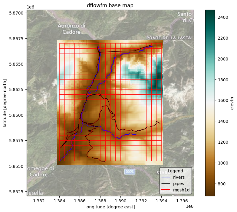
Plot model schematization base maps#
Here we plot the model base mesh information as well as the topography map.
[5]:
# we assume the model maps are in the projected CRS EPSG:3857
proj = ccrs.epsg(3857)
# adjust zoomlevel and figure size to your basis size & aspect
zoom_level = 12
figsize = (10, 8)

# initialize image with geoaxes
fig = plt.figure(figsize=figsize)
ax = fig.add_subplot(projection=proj)
bbox = elv.raster.box.to_crs(3857).buffer(3e3).to_crs(elv.raster.crs).total_bounds
extent = np.array(bbox)[[0, 2, 1, 3]]
ax.set_extent(extent, crs=proj)

# add sat background image
ax.add_image(cimgt.QuadtreeTiles(), zoom_level, alpha=0.5)

## plot elevation\
elv.plot(transform=proj, ax=ax, zorder=0.5, cmap="BrBG", add_colorbar=True)

# plot rivers
rivers.plot(ax=ax, linewidth= 1, color="blue", zorder=3, label="rivers")
# plot pipes
pipes.plot(ax=ax, color="k", linewidth=1, zorder=3, label="pipes")

## plot mesh
mesh1d.plot(ax=ax, color="r", zorder=2, label="mesh1d")
mesh2d.plot(ax=ax, facecolor="none", edgecolor="r", linewidth=0.5, zorder=2, label="mesh2d")

ax.xaxis.set_visible(True)
ax.yaxis.set_visible(True)
ax.set_ylabel(f"latitude [degree north]")
ax.set_xlabel(f"longitude [degree east]")
_ = ax.set_title(f"dflowfm base map")
legend = ax.legend(
    title="Legend",
    loc="lower right",
    frameon=True,
    framealpha=0.7,
    edgecolor="k",
    facecolor="white",
)

# save figure
# NOTE create figs folder in model root if it does not exist
# fn_out = join(mod.root, "figs", "basemap.png")
# plt.savefig(fn_out, dpi=225, bbox_inches="tight")
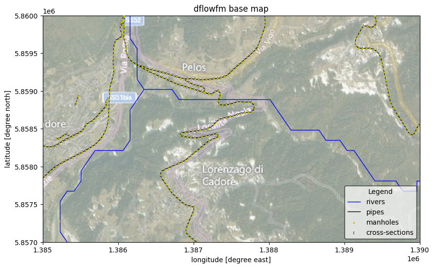
And zoom in to see better some of the structures:
[6]:
# we assume the model maps are in the projected CRS EPSG:3857
proj = ccrs.epsg(3857)
# adjust zoomlevel and figure size to your basis size & aspect
zoom_level = 14
figsize = (10, 8)
#extent = np.array([1385000, 1390000, 5861000, 5863000])
extent = np.array([1385000, 1390000, 5857000, 5860000])

# initialize image with geoaxes
fig = plt.figure(figsize=figsize)
ax = fig.add_subplot(projection=proj)
ax.set_extent(extent, crs=proj)

# add sat background image
ax.add_image(cimgt.QuadtreeTiles(), zoom_level, alpha=0.5)

# plot rivers
rivers.plot(ax=ax, linewidth= 1, color="blue", zorder=2, label="rivers")
# plot pipes
pipes.plot(ax=ax, color="k", linewidth=1, zorder=2, label="pipes")

# plot structures
manholes.plot(ax=ax, facecolor="y", markersize=2, zorder=4, label="manholes")
crosssections.plot(ax=ax, facecolor="grey", marker = '|',  markersize=15, zorder=3, label="cross-sections")

ax.xaxis.set_visible(True)
ax.yaxis.set_visible(True)
ax.set_ylabel(f"latitude [degree north]")
ax.set_xlabel(f"longitude [degree east]")
_ = ax.set_title(f"dflowfm base map")
legend = ax.legend(
    title="Legend",
    loc="lower right",
    frameon=True,
    framealpha=0.7,
    edgecolor="k",
    facecolor="white",
)