


Connecting D-SheetPiling to the probabilistic library#
Introduction#
This tutorial demonstrates how to connect a D-SheetPiling model to the probabilistic library to perform a FORM (First Order Reliability Method) analysis. The connection is made through the D-GEOLib Python library, which provides a programmatic interface to D-SheetPiling.
The workflow consists of three steps:
Build (or load) a D-SheetPiling model using D-GEOLib (tested with version 2.8.0)
Wrap it in a Python function that the probabilistic library can call as a limit state function
Parametrize the stochastic variables.
Run the FORM analysis and interpret the results
Inspect and post-process the results
Problem description#
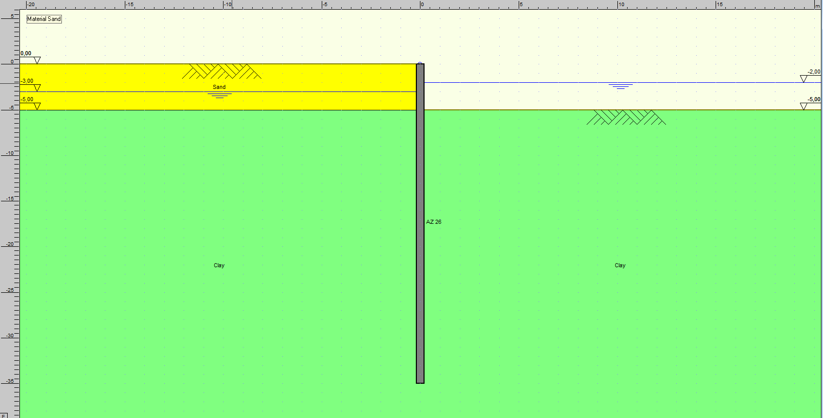
We consider a cantilever sheet pile wall along a canal in a two-layer soil profile:
Sand (top layer, 0.0 to −5.0 m NAP) — a medium-dense sand whose strength is governed by its friction angle \(\phi\)
Clay (bottom layer, −5.0 m NAP and below) — a soft clay whose strength is governed by its undrained shear strength \(S_u\)
The wall retains ground on the left side (ground level at 0.0 m NAP) against the canal on the right side (canal bed at −5.0 m NAP, canal water level at −2.0 m NAP). A phreatic surface is present behind the wall on the retained side.
The limit state function compares the maximum bending moment computed by D-SheetPiling against the moment capacity of the sheet pile section:
Failure occurs when \(g \leq 0\) (the calculated moment exceeds the section capacity).
Stochastic variables#
Variable |
Description |
Unit |
Distribution |
Mean |
CoV |
|---|---|---|---|---|---|
|
Friction angle of the sand layer |
° |
Normal |
25 |
0.10 |
|
Undrained shear strength of the clay layer |
kPa |
Log-normal |
20 |
0.10 |
|
Phreatic level behind the wall (retained side) |
m NAP |
Uniform |
[−4.0, −2.0] |
— |
First, let’s import the necessary packages to run this example. You need a Python environment with the GEOLIB library ( pip install d-geolib) installed to make run the following cells.
[1]:
from geolib.models.dsheetpiling import DSheetPilingModel
from geolib.models.dsheetpiling.constructions import Sheet, SheetPileProperties
from geolib.models.dsheetpiling.dsheetpiling_model import SheetModelType
from geolib.models.dsheetpiling.profiles import SoilProfile, SoilLayer
from geolib.models.dsheetpiling.settings import (
    LateralEarthPressureMethod,
    LateralEarthPressureMethodStage,
    Side,
    PassiveSide,
)
from geolib.models.dsheetpiling.water_level import WaterLevel
from geolib.geometry.one import Point
from geolib.soils import Soil
from geolib.models.dsheetpiling.surface import Surface

from probabilistic_library import ReliabilityProject, DistributionType, ReliabilityMethod, StandardNormal

import copy
import numpy as np
import matplotlib.pyplot as plt
from pathlib import Path
import tempfile
Step 1 — Build the D-SheetPiling base model (optional)#
We first create a deterministic D-SheetPiling model that represents the mean (baseline) configuration. This model will be modified at each iteration of the FORM algorithm, substituting the stochastic parameter values provided by the probabilsitic library.
Tip: If you already have a
.shifile, you can load it directly withmodel.parse("path/to/file.shi")instead of building it from scratch and fast-forward to step 2.
1.1 — Create the model and set the calculation method#
[2]:
base_model = DSheetPilingModel()

console_path = Path(r"C:\Program Files (x86)\Deltares\D-Sheet Piling 24.1.1\DSheetPiling.exe")
base_model.set_meta_property("dsheetpiling_console_path", console_path)

# Use the KA-KO-KP earth pressure method for sheet piling
base_model.set_model(SheetModelType(method=LateralEarthPressureMethod.C_PHI_DELTA))
base_model.datastructure.input_data.model.check_vertical_balance = False
1.2 — Define the soils#
We define two soil layers:
Sand — a frictional material (φ = 30°, c = 0)
Clay — a cohesive material modelled with undrained shear strength (φ = 0°, c = S_u = 25 kPa)
These properties are overwritten at each FORM iteration with the stochastic parameter values defined in the model.
[3]:
# Sand layer (frictional)
sand = Soil(name="Sand")
sand.soil_weight_parameters.saturated_weight = 20.0        # saturated unit weight [kN/m³]
sand.soil_weight_parameters.unsaturated_weight = 17.0        # dry unit weight [kN/m³]
sand.mohr_coulomb_parameters.friction_angle = 25.0           # friction angle [°] will be overwritten in the limit state function to introduce uncertainty
sand.mohr_coulomb_parameters.cohesion = 0.0       # cohesion [kPa]
sand.mohr_coulomb_parameters.friction_angle_interface = 20.0         # wall friction angle [°]
base_model.add_soil(sand)

# Clay layer (cohesive, undrained)
clay = Soil(name="Clay")
clay.soil_weight_parameters.saturated_weight = 18.0        # saturated unit weight [kN/m³]
clay.soil_weight_parameters.unsaturated_weight = 16.0        # dry unit weight [kN/m³]
clay.mohr_coulomb_parameters.friction_angle = 0.0            # friction angle [°] (undrained: φ = 0)
clay.mohr_coulomb_parameters.cohesion = 20.0      # undrained shear strength Su [kPa] will be overwritten in the limit state function to introduce uncertainty
clay.mohr_coulomb_parameters.friction_angle_interface = 0.0          # wall friction angle [°]
base_model.add_soil(clay)
[3]:
'Clay'
1.3 — Define the sheet pile construction#
We place a sheet pile wall with its top at 0.0 m NAP and a bottom at −35.0 m NAP. The section has an elastic stiffness EI = 50 000 kNm²/m and a characteristic elastic moment capacity of M_capacity = 500 kNm/m.
[4]:
# Moment capacity of the sheet pile section [kNm/m]
M_CAPACITY = 500.0

sheet = Sheet(
    name="AZ 26",
    sheet_pile_properties=SheetPileProperties(
        elastic_stiffness_ei=50000,          # EI [kNm²/m]
        section_bottom_level=-35.0,          # bottom of the sheet pile [m NAP]
        mr_char_el=M_CAPACITY,               # characteristic elastic moment capacity [kNm/m]
    ),
)
base_model.set_construction(top_level=0.0, elements=[sheet])
1.4 — Define the construction stage#
A single construction stage with:
Left (retained) side: ground level at 0.0 m NAP, Sand from 0.0 to −5.0 m, Clay below −5.0 m. Phreatic level at −1.0 m NAP.
Right (canal) side: canal bed at −5.0 m NAP, Clay below −5.0 m. Canal water level at −2.0 m NAP.
[5]:
# Add a construction stage
stage_id = base_model.add_stage(
    name="Canal",
    passive_side=PassiveSide.DSHEETPILING_DETERMINED,
    method_left=LateralEarthPressureMethodStage.C_PHI_DELTA,
    method_right=LateralEarthPressureMethodStage.C_PHI_DELTA,
)

# Add a new surface object at the retained side
surface_left = Surface(name="Surface_left", points=[Point(x=0.0, z=0.0)])
base_model.add_surface(surface_left, side=Side.LEFT, stage_id=stage_id)

# Left side (retained): Sand 0.0 to -5.0 m, Clay below -5.0 m
profile_left = SoilProfile(
    name="Left",
    layers=[
        SoilLayer(top_of_layer=0.0, soil="Sand"),
        SoilLayer(top_of_layer=-5.0, soil="Clay"),
    ],
    coordinate=Point(x=0.0),
)
base_model.add_profile(profile_left, side=Side.LEFT, stage_id=stage_id)

# Phreatic level behind the wall (retained side) at -1.0 m NAP
wl_left = WaterLevel(name="WL_left", level=-1.0)
base_model.add_head_line(wl_left, side=Side.LEFT, stage_id=stage_id)

bottom_depth = -5.0

# Add a new surface object at the canal side
surface_right = Surface(name="Surface_right", points=[Point(x=0.0, z=bottom_depth)])
base_model.add_surface(surface_right, side=Side.RIGHT, stage_id=stage_id)

profile_right = SoilProfile(
    name="Right",
    layers=[
        SoilLayer(top_of_layer=bottom_depth, soil="Clay"),
    ],
    coordinate=Point(x=0.0, z=bottom_depth),
)
base_model.add_profile(profile_right, side=Side.RIGHT, stage_id=stage_id)

# Canal water level
wl_right = WaterLevel(name="WL_right", level=-2.0)
base_model.add_head_line(wl_right, side=Side.RIGHT, stage_id=stage_id)
Alternative: Loading an existing .shi file#
If you already have a D-SheetPiling input file, the setup simplifies to:
base_model = DSheetPilingModel()
base_model.parse(Path("path/to/your_model.shi"))
The rest of the workflow (defining the wrapper function, setting up the reliability project, running FORM) remains identical. The only thing that changes is how you update the stochastic parameters inside the limit state function — you need to locate the correct soil or water level object in the parsed data structure.
Step 2 — Define the limit state function#
The limit state function is a regular Python function whose argument names must match the variable names used in the project object of the probabilistic library. At each FORM iteration the probabilistic library calls this function with a new set of parameter values.
Inside the function we:
Deep-copy the base model so the original is not modified
Update the stochastic parameters (soil properties, phreatic level)
Serialize the model to a
.shifile and Execute D-SheetPilingExtract the maximum bending moment from the output
Return \(g = M_{\text{capacity}} - |M_{\text{max}}|\)
[6]:
i = 1
[7]:
# Working directory for temporary .shi files
WORK_DIR = Path(tempfile.mkdtemp(prefix="dsheet_ptk_")).resolve()

def lsf_sheetpile(phi_sand, su_clay, phreatic_level):
    """
    Limit state function: g = M_capacity - |M_max|

    Parameters
    ----------
    phi_sand : float
        Friction angle of the sand layer [°].
    su_clay : float
        Undrained shear strength of the clay layer [kPa].
    phreatic_level : float
        Phreatic level behind the wall (retained side) [m NAP].
    """
    global i

    # 1. Deep-copy the base model
    model = copy.deepcopy(base_model)

    # Add a safeguard against too low strength values, they could make DSheet-piling crash and we consider them as failed anyway.
    if phi_sand <= 5.0 or su_clay <= 5.0:
        return 0

    # 2. Update stochastic soil parameters
    #    Soil[0] = Sand, Soil[1] = Clay (order follows add_soil calls)
    soils = model.datastructure.input_data.soil_collection.soil

    # Sand: update friction angle and wall friction (δ = 2/3 × φ)
    soils[0].soilphi = phi_sand
    soils[0].soildelta = 2 / 3 * phi_sand

    # Clay: update undrained shear strength (entered as cohesion with φ = 0)
    soils[1].soilcohesion = su_clay

    #. Update the phreatic level on the retained side
    model.datastructure.input_data.waterlevels.levels[0].level = phreatic_level

    # 3. Serialize and execute
    shi_path = WORK_DIR / f"model_{i}.shi"
    i += 1

    model.serialize(shi_path)
    model.execute()

    # 4. Extract maximum bending moment from the output
    stage_output = model.output.construction_stage[0]
    mfd = stage_output.moments_forces_displacements.momentsforcesdisplacements
    max_moment = max(abs(row["moment"]) for row in mfd)

    # 5. Return the limit state value
    g = M_CAPACITY - max_moment

    return g
Key points about the wrapper function#
The function signature
lsf_sheetpile(phi_sand, su_clay, phreatic_level)defines the stochastic variables. The probabilistic library uses introspection on the function arguments to automatically register them.Each call to the function creates a fresh copy of the base model (
copy.deepcopy), updates the relevant parameters, and runs D-SheetPiling. This ensures that each FORM iteration is independent.The soil objects in
model.datastructure.input_data.soil_collection.soilare indexed in the order they were added:soil[0]= Sand,soil[1]= Clay.The function must return a scalar value: the limit state value \(g\). The sign convention is \(g > 0\) (safe) and \(g \leq 0\) (failure).
D-SheetPiling must be installed on the machine and accessible via the default console path (or set
model.custom_console_path).
Step 3 — Set up the Reliability Project#
We create a ReliabilityProject, assign the limit state function as the model, and define the stochastic variables with their distributions.
[8]:
project = ReliabilityProject()
project.model = lsf_sheetpile
Define the stochastic variables#
Each argument of lsf_sheetpile is automatically available as a variable in project.variables. We specify the marginal distribution, mean, and either the coefficient of variation (variation) or the standard deviation (deviation).
Note that su_clay uses a log-normal distribution, which is common for undrained shear strength as it is strictly positive and typically right-skewed. The phreatic_level uses a uniform distribution to represent the range of groundwater levels behind the wall.
[9]:
# Friction angle of sand: Normal(mean=25°, CoV=0.10)
project.variables["phi_sand"].distribution = DistributionType.normal
project.variables["phi_sand"].mean = 25.0
project.variables["phi_sand"].variation = 0.10

# Undrained shear strength of clay: Log-normal(mean=20 kPa, CoV=0.10)
project.variables["su_clay"].distribution = DistributionType.log_normal
project.variables["su_clay"].mean = 20.0
project.variables["su_clay"].variation = 0.10

# Phreatic level behind the wall: Uniform(lower=-4.0, upper=-2.0)
project.variables["phreatic_level"].distribution = DistributionType.uniform
project.variables["phreatic_level"].minimum = -4.0
project.variables["phreatic_level"].maximum = -2.0
Step 4 — Run the FORM analysis#
We configure the FORM settings and run the analysis. The relaxation_factor controls the step size in the algorithm; a smaller value improves stability for models with a non-smooth response surface but makes convergence slower. The convergence threshold can also be modified the parameter epsilon_beta.
For more details about the FORM procedure, please refer to the scientific documentation.
[10]:
project.settings.reliability_method = ReliabilityMethod.form

project.settings.maximum_iterations = 80
project.settings.relaxation_factor = 0.15
project.settings.step_size = 0.05  # Step size for finite difference approximation of the reliability index gradient
project.settings.epsilon_beta = 0.05  # This is the convergence criterion for the reliability index β (stop if |β_new - β_old| < ε_β)

# Save intermediate results for plotting
project.settings.save_convergence = True
project.settings.save_realizations = True

project.run()
Added 2 lines to run_identification.
Added 2 lines to run_identification.
Added 2 lines to run_identification.
Added 2 lines to run_identification.
Added 2 lines to run_identification.
Added 2 lines to run_identification.
Added 2 lines to run_identification.
Added 2 lines to run_identification.
Added 2 lines to run_identification.
Added 2 lines to run_identification.
Added 2 lines to run_identification.
Added 2 lines to run_identification.
Added 2 lines to run_identification.
Added 2 lines to run_identification.
Added 2 lines to run_identification.
Added 2 lines to run_identification.
Added 2 lines to run_identification.
Added 2 lines to run_identification.
Added 2 lines to run_identification.
Added 2 lines to run_identification.
Added 2 lines to run_identification.
Added 2 lines to run_identification.
Added 2 lines to run_identification.
Added 2 lines to run_identification.
Added 2 lines to run_identification.
Added 2 lines to run_identification.
Added 2 lines to run_identification.
Added 2 lines to run_identification.
Added 2 lines to run_identification.
Added 2 lines to run_identification.
Added 2 lines to run_identification.
Added 2 lines to run_identification.
Added 2 lines to run_identification.
Added 2 lines to run_identification.
Added 2 lines to run_identification.
Added 2 lines to run_identification.
Added 2 lines to run_identification.
Added 2 lines to run_identification.
Added 2 lines to run_identification.
Added 2 lines to run_identification.
Added 2 lines to run_identification.
Added 2 lines to run_identification.
Added 2 lines to run_identification.
Added 2 lines to run_identification.
Added 2 lines to run_identification.
Added 2 lines to run_identification.
Added 2 lines to run_identification.
Added 2 lines to run_identification.
Added 2 lines to run_identification.
Added 2 lines to run_identification.
Added 2 lines to run_identification.
Added 2 lines to run_identification.
Added 2 lines to run_identification.
Added 2 lines to run_identification.
Added 2 lines to run_identification.
Added 2 lines to run_identification.
Added 2 lines to run_identification.
Added 2 lines to run_identification.
Added 2 lines to run_identification.
Added 2 lines to run_identification.
Added 2 lines to run_identification.
Added 2 lines to run_identification.
Added 2 lines to run_identification.
Added 2 lines to run_identification.
Added 2 lines to run_identification.
Added 2 lines to run_identification.
Added 2 lines to run_identification.
Added 2 lines to run_identification.
Added 2 lines to run_identification.
Added 2 lines to run_identification.
Added 2 lines to run_identification.
Added 2 lines to run_identification.
Added 2 lines to run_identification.
Added 2 lines to run_identification.
Added 2 lines to run_identification.
Added 2 lines to run_identification.
Added 2 lines to run_identification.
Added 2 lines to run_identification.
Added 2 lines to run_identification.
Added 2 lines to run_identification.
Step 5 — Read the results#
After the FORM analysis converges, the design point contains:
β — the reliability index
P_f — the probability of failure
α-factors — the influence coefficients showing each variable’s contribution
Design-point values — the parameter values at the most likely failure point
[11]:
project.design_point.print()
Reliability (FORM)
 Reliability index = 1.876
 Probability of failure = 0.0303
 Convergence = 0.04096 (converged)
 Model runs = 80
Alpha values:
 phi_sand: alpha = 0.2015, x = 24.05
 su_clay: alpha = 0.9114, x = 16.78
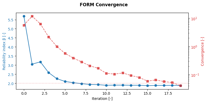
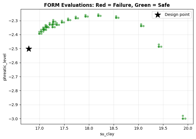
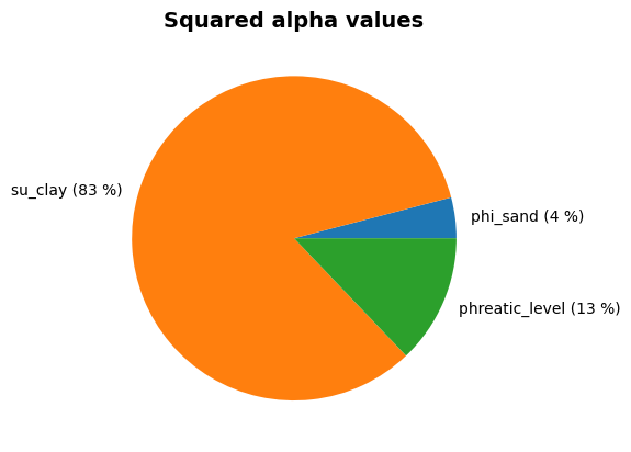
 phreatic_level: alpha = -0.3589, x = -2.501
Tip: The D-Sheetpiling files are saved for every iteration (model_i.shi and model_i.shd) which allows for further control. They can be found in the folder defined as WORK_DIR. It is important to manually check if the values for the stochastic parameters have been correctly written in the file and are physically possible (no negative friction angle for example).
Step 6 — Visualise the results#
6.1 — FORM convergence#
The convergence plot shows the reliability index \(\beta\) and the convergence criterion as a function of the FORM iteration number. A stable, converging \(\beta\) confirms that the algorithm has found a consistent design point.
[13]:
dp = project.design_point

iterations = [r.index for r in dp.reliability_results]
betas = [r.reliability_index for r in dp.reliability_results]
convergences = [r.convergence for r in dp.reliability_results]

fig, ax1 = plt.subplots(figsize=(8, 4))

color_beta = "tab:blue"
ax1.set_xlabel("Iteration [-]")
ax1.set_ylabel("Reliability index β [-]", color=color_beta)
ax1.plot(iterations, betas, "o-", color=color_beta, label="β")
ax1.tick_params(axis="y", labelcolor=color_beta)

ax2 = ax1.twinx()
color_conv = "tab:red"
ax2.set_ylabel("Convergence [-]", color=color_conv)
ax2.plot(iterations, convergences, "s--", color=color_conv, alpha=0.7, label="convergence")
ax2.axhline(project.settings.variation_coefficient, color=color_conv, linestyle=":", alpha=0.4, label="threshold")
ax2.tick_params(axis="y", labelcolor=color_conv)
ax2.set_yscale("log")

fig.suptitle("FORM Convergence", fontweight="bold")
fig.tight_layout()
plt.show()
6.2 — Design point in the variable domain#
The scatter plot below shows all model evaluations performed during the FORM iterations, projected onto the two most influential variables. The design point (black marker) is the most probable failure point. Red points indicate failure (\(g \leq 0\)), green points indicate safe evaluations (\(g > 0\)).
[14]:
# Identify the two most influential variables
influence = [alpha.influence_factor for alpha in dp.alphas]
idx_sorted = np.argsort(influence)
idx_x, idx_y = int(idx_sorted[-1]), int(idx_sorted[-2])

# Extract realization values
x_vals = [r.input_values[idx_x] for r in dp.realizations]
y_vals = [r.input_values[idx_y] for r in dp.realizations]
z_vals = [r.z for r in dp.realizations]
colors = ["red" if z <= 0 else "green" for z in z_vals]

fig, ax = plt.subplots(figsize=(7, 5))
ax.scatter(x_vals, y_vals, c=colors, alpha=0.5, edgecolors="none", s=30)
ax.scatter(
    dp.alphas[idx_x].x,
    dp.alphas[idx_y].x,
    marker="*", s=250, c="black", zorder=5, label="Design point",
)
ax.set_xlabel(dp.alphas[idx_x].identifier)
ax.set_ylabel(dp.alphas[idx_y].identifier)
ax.legend()
ax.set_title("FORM Evaluations: Red = Failure, Green = Safe", fontweight="bold")
ax.grid(True, alpha=0.3)
fig.tight_layout()
plt.show()
6.3 — Influence factors (pie chart)#
The influence factor of each variable equals \(\alpha^2\); all influence factors sum to 1. The pie chart shows at a glance which uncertain parameters dominate the failure probability and where further investigation or risk reduction measures would be most effective.
[15]:
project.design_point.plot_alphas()
Interpretation#
The α-factors indicate the relative importance of each variable in driving the failure probability:
A large |α| for
phi_sandmeans the sand friction angle dominates the uncertainty — investing in better soil investigation of the sand layer would be the most effective way to reduce uncertainty.A large |α| for
su_clayindicates that the clay strength is a critical parameter. This is expected for configurations where the sheet pile toe is embedded in clay below the canal bed.A large |α| for
phreatic_levelsuggests that the groundwater level behind the wall relative to the canal water level is an important driver. Controlling seepage or drainage on the retained side would reduce uncertainty.The sign of α indicates the direction: a positive α means the variable contributes to resistance (increasing it makes the structure safer), while a negative α means it contributes to loading.
The design-point values \(x^*\) represent the most probable combination of parameter values that leads to failure. These can be compared to the characteristic or design values used in semi-probabilistic codes (e.g., Eurocode 7) as a consistency check.
Credits: Thanks to Antonis Mavritsakis (Deltares)